Inference Methods and Parameter Estimation Techniques

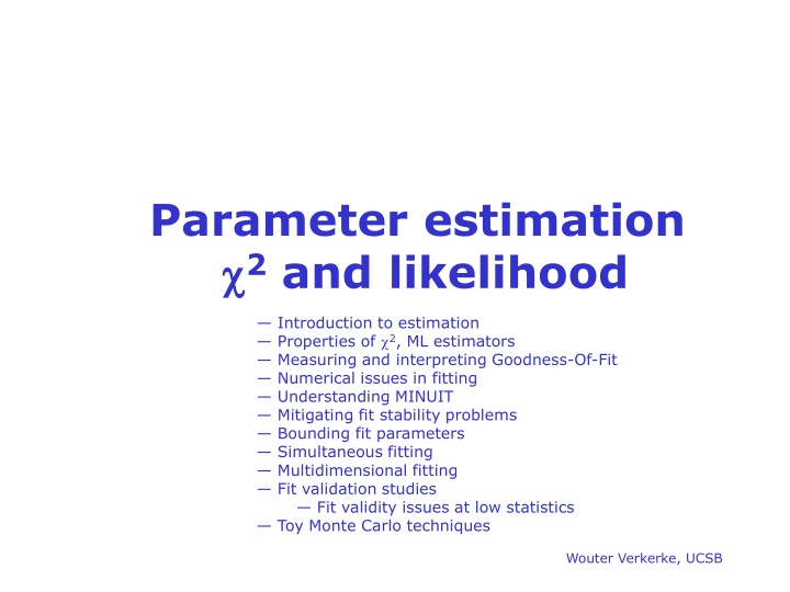
Parameter estimation 2 and likelihood Introduction to estimation Properties of 2, ML estimators Measuring and interpreting Goodness-Of-Fit Numerical issues in fitting Understanding MINUIT Mitigating fit stability problems Bounding fit parameters Simultaneous fitting Multidimensional fitting Fit validation studies Fit validity issues at low statistics Toy Monte Carlo techniques Wouter Verkerke, UCSB

Parameter estimation Introduction D ( ; ) (x ) T x p Probability Theory Data Calculus Given the theoretical distribution parameters p, what can we say about the data ) (x D ( ; ) T x p Data Theory Statistical inference Need a procedure to estimate p from D Wouter Verkerke, UCSB

Multiple methods Many ways to infer information on model (parameter) from data 2 fit p = 5.2 0.3 Likelihood fit p = 4.7 0.4 Bayesian interval p [ 4.5 5.9 ] at 68% credibility Frequentist interval p [ 4.4 5.8 ] at 68% confidence level When data is abundant, methods usually give consistent answers Issues and differences between methods arise when experimental result contains little information Easy Difficult Wouter Verkerke, NIKHEF

Multiple methods Many ways to infer information on model (parameter) from data 2 fit p = 5.2 0.3 Likelihood fit p = 4.7 0.4 Bayesian interval p [ 4.5 5.9 ] at 68% credibility Frequentist interval p [ 4.4 5.8 ] at 68% confidence level Will first focus 2 and likelihood estimation procedures Well known, often used Explore assumptions, limitations Later we focus on interpreting experiments with little information content Wouter Verkerke, NIKHEF

Basics What is an estimator? An estimator is a procedure giving a value for a parameter or a property of a distribution as a function of the actual data values, i.e. i N 1 ) ( Estimator of the variance 1 ( = ) x x Estimator of the mean i i = 2) ( V x x i N A perfect estimator is = ) ( lim a a Consistent: n Unbiased With finite statistics you get the right answer on average This is called the Minimum Variance Bound = 2) ) ( a V ( a a Efficient There are no perfect estimators for most problems Wouter Verkerke, UCSB

How to model your data Approach in 2 fit very empirical Function f(x,y) can be any arbitrary function Many techniques (Likelihood, Bayesian, Frequentist) require a more formal approach to data modeling through probability density functions We can characterize data distributions with probability density functions F(x;p) x = observables (measured quantities) p = parameters (model/theory parameters) Properties Normalized to unity with respect to observable(s) x Positive definite F(x;p)>=0 for all (x,p) F 1 ( ; ) F x p d x ( ; ) 0 x p Wouter Verkerke, NIKHEF 1 ) dxdy y ( , F x 1 ( ) F x dx

Probability density functions Properties Parameters can be physics quantities of interest (life time, mass) Invariant mass distribution observable x (inv. mass) parameter m (physics mass) parameter (decay width) Decay time distribution observable x (decay time) parameter (lifetime) 2 x 1 1 m = ( ; ) exp f x m 2 2 Vehicle to infer physics parameters from data distributions Wouter Verkerke, NIKHEF

Likelihood The likelihood is the value of a probability density function evaluated at the measured value of the observable(s) Note that likelihood is only function of parameters, not of observables = ( ) ( ; ) L p F x x p data For a dataset that consists of multiple data points, the product is taken = = ( ) ( ; , ) p i.e. ( ) ( ; ) ( ; ) ( ; )... L p F x L p F x p F x p F x p 0 1 2 i i Wouter Verkerke, NIKHEF

Probability, Probability Density, and Likelihood For discrete observables we have probabilities instead of probability densities Unit Normalization requirement still applies Poisson probability P(n| ) = nexp(- )/n! Gaussian probability density function (pdf) p(x| , ): p(x| , )dx is differential of probability dP. In Poisson case, suppose n=3 is observed. Substituting n=3 into P(n| ) yields the likelihood function L( ) = 3exp(- )/3! Key point is that L( ) is nota probability density in . (It is not a density!) Area under L is meaningless. That s why a new word, likelihood , was invented for this function of the parameter(s), to distinguish from a pdf in the observable(s)! Many people nevertheless talk about integrating the likelihood confusion about what is done in Bayesian interval (more later) Likelihood Ratios L( 1) /L( 2) are useful and frequently used. Wouter Verkerke, NIKHEF

Change of variable x, change of parameter For pdf p(x| ) and (1-to-1) change of variable from x to y(x): p(y(x)| ) = p(x| ) / |dy/dx|. Jacobian modifies probability density, guarantees that P( y(x1)< y < y(x2) ) = P(x1< x < x2), i.e., that Probabilities are invariant under change of variable x. Mode of probability density is not invariant (so, e.g., criterion of maximum probability density is ill-defined). Likelihood ratio is invariant under change of variable x. (Jacobian in denominator cancels that in numerator). For likelihood L( ) and reparametrization from to u( ): L( ) = L(u( )) (!). Likelihood L( ) is invariant under reparametrization of parameter (reinforcing fact that L is not a pdf in ). Wouter Verkerke, NIKHEF

Parameter estimation using Maximum Likelihood Likelihood is high for values of p that result in distribution similar to data Define the maximum likelihood (ML) estimator(s) to be the parameter value(s) for which the likelihood is maximum. Wouter Verkerke, NIKHEF

Parameter estimation Maximum likelihood Computational issues For convenience the negative log of the Likelihood is often used as addition is numerically easier than multiplication i = ln ( ) ln ( ip x ; ) L p F Maximizing L(p) equivalent to minimizing log L(p) In practice, find point where derivative is zero ln ( ) d L p = 0 d p = p p i i Wouter Verkerke, UCSB

Variance on ML parameter estimates The ML estimator for the parametervariance is 1 2 ln d L From Rao-Cramer-Frechet inequality ( V ( = = 2 ) ) p p 2 d p + 1 db ( ) p ) ( V dp 2ln d L 2 d p I.e. variance is estimated from 2nd derivative of log(L) at minimum b = bias as function of p, inequality becomes equality in limit of efficient estimator Valid if estimator is efficient and unbiased! Visual interpretation of variance estimate Taylor expand log(L) around minimum -log(L) 0.5 2 ln dp ln 2 d L d L = + + 2 ) ( p L ) p ) p ln ( ) ln ( ( L p p p 1 2 d p = = p p p p p 2 2 ) p ln 2 ( d L p = + ln L max 2 d p = p p 2 ) 2 p ( 1 p p = + = ln ln ( ) ln L L p L p max max Wouter Verkerke, UCSB 2 2

Properties of Maximum Likelihood estimators In general, Maximum Likelihood estimators are Consistent (gives right answer for N ) Mostly unbiased (bias 1/N, may need to worry at small N) Efficient for large N (you get the smallest possible error) ( ) p Invariant: (a transformation of parameters will Not change your answer, e.g Use of 2nd derivative of log(L) for variance estimate is usually OK ( ) p 2 = 2 MLE efficiency theorem: the MLE will be unbiased and efficient if an unbiased efficient estimator exists Proof not discussed here Of course this does not guarantee that any MLE is unbiased and efficient for any given problem Wouter Verkerke, UCSB

More about maximum likelihood estimation It s not right it is just sensible It does not give you the most likely value of p it gives you the value of p for which this data is most likely Numeric methods are often needed to find the maximum of ln(L) Especially difficult if there is >1 parameter Standard tool in HEP: MINUIT (more about this later) Max. Likelihood does not give you a goodness-of-fit measure If assumed F(x;p) is not capable of describing your data for any p, the procedure will not complain The absolute value of L tells you nothing! Wouter Verkerke, UCSB

Relation between Likelihood and 2 estimators Properties of 2 estimator follow from properties of ML estimator using Gaussian probability density functions Probability Density Function in p for single data point xi( i) and function f(xi;p) 2 ( ; ) y f x p = ( , , ; ) exp i i F x y p i i i i Take log, Sum over all points (xi ,yi , i) ( ; ) y f x p The Likelihood function in p for given points xi( i) and function f(xi;p) i = = 2 ln ( ) L p i i 1 1 2 2 i The 2 estimator follows from ML estimator, i.e it is Efficient, consistent, bias 1/N, invariant, But only in the limit that the error on xi is truly Gaussian i.e. need ni > 10 if yi follows a Poisson distribution Bonus: Goodness-of-fit measure 2 1 per d.o.f Wouter Verkerke, UCSB

Example of 2 vs ML fit Example with many low statistics bins true distribution 2 fit unbinned ML fit binned ML fit Wouter Verkerke, NIKHEF

Example of binned vs unbinned ML fit Lowering number of bins and number of events true distribution unbinned ML fit binned ML fit Proper way to study bias, precision is with toy MC study at the end of this module Wouter Verkerke, NIKHEF

Maximum Likelihood or 2 What should you use? 2 fit is fastest, easiest Works fine at high statistics Gives absolute goodness-of-fit indication Make (incorrect) Gaussian error assumption on low statistics bins Has bias proportional to 1/N Misses information with feature size < bin size Full Maximum Likelihood estimators most robust No Gaussian assumption made at low statistics No information lost due to binning Gives best error of all methods (especially at low statistics) No intrinsic goodness-of-fit measure, i.e. no way to tell if best is actually pretty bad Has bias proportional to 1/N Can be computationally expensive for large N bins = Binned Maximum Likelihood in between Much faster than full Maximum Likihood Correct Poisson treatment of low statistics bins Misses information with feature size < bin size Has bias proportional to 1/N ln ( ) ln ( ; ) L p n F x p binned bin bin center Wouter Verkerke, UCSB

You can (almost) always avoid 2 fits Case study: Fit for efficiency function Have some simulation sample: need to parameterize which fraction of events passes as function of observable x Traditional 2approach Make histogram of Npassed/Ntotal Fit parameterized efficiency function to histogram Tricky question: what errors to use? N is wrong. = = ( ) 1 ( ) 1 ( ) V r np p np p Can use binomial errors However still quite approximate: true errors will be asymmetric (i.e. no upward error on bin with Npass=10, Ntotal=10) Wouter Verkerke, NIKHEF

You can (almost) always avoid 2 fits MLE approach Realize that your dataset has two observables (x,c), where c is a discrete observable with states accept and reject Corresponding probability density function: = = + ( | , ) ( ) ( , x ) p F c x p c accept x p = ( )( 1 ( , )) c reject Clearly unit-normalized over c for each value of (x,p) ( must be between 0 and 1 for all (x,p)) Write log(L) as usual, using above p.d.f. and minimize i = ln ( ) ln ( , ; ) L p F x c p i i Result: estimation of e(x,p) using correct binomial/poisson assumption on distribution of observables. Fit can also be performed unbinned Wouter Verkerke, NIKHEF

You can (almost) always avoid 2 fits Example of unbinned MLE fit for efficiency Wouter Verkerke, NIKHEF

Weighted data Sometimes input data is weighted Examples: Certain Next-to-leading order event generator for LHC physics produce simulated events with weights +1 and -1. You ve subtracted a distribution of background events from a sideband in data (also results in events with weight +1 and -1) You work with reweighted data samples for a variety of reasons (e.g. not enough data was available for one background sample, rescale available events with some non-unit weight to match available amounts of other samples) How to deal with event weights in 2, MLE parameter estimation 2 fit of histograms with weighted data are straightforward From C.L.T 2 ( ; ) y f x p i i 1 = 2 = i i = y w i w2 i i i i i From C.L.T ( V ( p ) ) p NB: You may no longer be able to interpret as a Gaussian error (i.e. 68% contained in 1 ) Wouter Verkerke, NIKHEF

Weighted data 2 vs MLE Adding event weights to log(L) straightforward, but does not yield correct estimates on parameter variance Event weight i = ln ( ) ln ( ; ) L p w F x p weighted i i i i w Variance estimate on parameters will be proportional to N w i If errors will be too small, if errors will be too large! i i w N i No clean solution available that retains all good properties of MLE, but it is possible to perform sum-of-weights-like correction to covariance matrix to correct for effect of on-unit weights = 1 V VC V where V is the cov. matrix calculated from a log(L) with event weights w, and C is the cov. matrix calculated from a log(L) with event weights w2 It is easy to see that in the case of 1 parameter this is equivalent to 1 = i w2 i i Wouter Verkerke, UCSB

Hypothesis testing Goodness of fit Hypothesis testing and goodness-of-fit Reminder: classical hypothesis test compares data to two hypothesis H0 and H1 (e.g background-only vs signal+background). Type-I error = claiming signal when you should not have Type-II error = not claiming signal when you should have If there is no alternate (H0) hypothesis, hypothesis test is called goodness-of-fit test. NB: Can only quantify Type-I error thus question which g.o.f. test is best (e.g. 2, Kolmogorov) is ill posed Not a good fit Wouter Verkerke, NIKHEF

Estimating and interpreting Goodness-Of-Fit Most common test: the 2 test 2 ( ; ) y f x p i = 2 i i i If f(x) describes data then 2 N, if 2 >> N something is wrong How to quantify meaning of large 2 ? What you really want to know: the probability that a function which does genuinely describe the data on N points would give a 2 probability as large or larger than the one you already have. For large N, sqrt(2 2) has a Gaussian distribution with mean sqrt(2N-1) and =1 Easy How to make a well calibrated statement for intermediate N Wouter Verkerke, UCSB

How to quantify meaning of large 2 Probability distr. for 2 is given by 2 iy 2 = i i i / 2 N 2 2 = 2 2 / 2 N ( , ) p N e ( ) 2 / N Observed 2 for n=10 P = integral over shaded area = d 2 2 2 ( ; ) ( ; ' ) ' P N p N 2 Good news: Integral of 2 pdf is analytically calculable! Wouter Verkerke, UCSB

Goodness-of-fit 2 Example for 2 probability Suppose you have a function f(x;p) which gives a 2 of 20 for 5 points (histogram bins). Not impossible that f(x;p) describes data correctly, just unlikely 20 d = 2 2 ( ) 5 , 0012 . 0 p How unlikely? Note: If function has been fitted to the data Then you need to account for the fact that parameters have been adjusted to describe the data N N = N d.o.f . data params Practical tips To calculate the probability in ROOT TMath::Prob(chi2,ndf) Wouter Verkerke, UCSB

Practical estimation Numeric 2 and -log(L) minimization For most data analysis problems minimization of 2 or log(L) cannot be performed analytically Need to rely on numeric/computational methods In >1 dimension generally a difficult problem! But no need to worry Software exists to solve this problem for you: Function minimization workhorse in HEP many years: MINUIT MINUIT does function minimization and error analysis It is used in the PAW,ROOT fitting interfaces behind the scenes It produces a lot of useful information, that is sometimes overlooked Will look in a bit more detail into MINUIT output and functionality next Wouter Verkerke, UCSB

Numeric 2/-log(L) minimization Proper starting values For all but the most trivial scenarios it is not possible to automatically find reasonable starting values of parameters This may come as a disappointment to some So you need to supply good starting values for your parameters -log(L) Reason: There may exist multiple (local) minima in the likelihood or 2 Local minimum True minimum p Supplying good initial uncertainties on your parameters helps too Reason: Too large error will result in MINUIT coarsely scanning a wide region of parameter space. It may accidentally find a far away local minimum Wouter Verkerke, UCSB

Example of interactive fit in ROOT What happens in MINUIT behind the scenes 1) Find minimum in log(L) or 2 MINUIT function MIGRAD 2) Calculate errors on parameters MINUIT function HESSE 3) Optionally do more robust error estimate MINUIT function MINOS Wouter Verkerke, UCSB

Minuit function MIGRAD Purpose: find minimum Progress information, watch for errors here ********** ** 13 **MIGRAD 1000 1 ********** (some output omitted) MIGRAD MINIMIZATION HAS CONVERGED. MIGRAD WILL VERIFY CONVERGENCE AND ERROR MATRIX. COVARIANCE MATRIX CALCULATED SUCCESSFULLY FCN=257.304 FROM MIGRAD STATUS=CONVERGED 31 CALLS 32 TOTAL EDM=2.36773e-06 STRATEGY= 1 ERROR MATRIX ACCURATE EXT PARAMETER STEP FIRST NO. NAME VALUE ERROR SIZE DERIVATIVE 1 mean 8.84225e-02 3.23862e-01 3.58344e-04 -2.24755e-02 2 sigma 3.20763e+00 2.39540e-01 2.78628e-04 -5.34724e-02 ERR DEF= 0.5 EXTERNAL ERROR MATRIX. NDIM= 25 NPAR= 2 ERR DEF=0.5 1.049e-01 3.338e-04 3.338e-04 5.739e-02 PARAMETER CORRELATION COEFFICIENTS NO. GLOBAL 1 2 1 0.00430 1.000 0.004 2 0.00430 0.004 1.000 Parameter values and approximate errors reported by MINUIT Error definition (in this case 0.5 for a likelihood fit) Wouter Verkerke, UCSB

Minuit function MIGRAD Purpose: find minimum Value of 2 or likelihood at minimum ********** ** 13 **MIGRAD 1000 1 ********** (some output omitted) MIGRAD MINIMIZATION HAS CONVERGED. MIGRAD WILL VERIFY CONVERGENCE AND ERROR MATRIX. COVARIANCE MATRIX CALCULATED SUCCESSFULLY FCN=257.304 FROM MIGRAD STATUS=CONVERGED 31 CALLS 32 TOTAL EDM=2.36773e-06 STRATEGY= 1 ERROR MATRIX ACCURATE EXT PARAMETER STEP FIRST NO. NAME VALUE ERROR SIZE DERIVATIVE 1 mean 8.84225e-02 3.23862e-01 3.58344e-04 -2.24755e-02 2 sigma 3.20763e+00 2.39540e-01 2.78628e-04 -5.34724e-02 ERR DEF= 0.5 EXTERNAL ERROR MATRIX. NDIM= 25 NPAR= 2 ERR DEF=0.5 1.049e-01 3.338e-04 3.338e-04 5.739e-02 PARAMETER CORRELATION COEFFICIENTS NO. GLOBAL 1 2 1 0.00430 1.000 0.004 2 0.00430 0.004 1.000 (NB: 2 values are not divided by Nd.o.f) Approximate Error matrix And covariance matrix Wouter Verkerke, UCSB

Minuit function MIGRAD Status: Should be converged but can be failed Purpose: find minimum Estimated Distance to Minimum should be small O(10-6) ********** ** 13 **MIGRAD 1000 1 ********** (some output omitted) MIGRAD MINIMIZATION HAS CONVERGED. MIGRAD WILL VERIFY CONVERGENCE AND ERROR MATRIX. COVARIANCE MATRIX CALCULATED SUCCESSFULLY FCN=257.304 FROM MIGRAD STATUS=CONVERGED 31 CALLS 32 TOTAL EDM=2.36773e-06 STRATEGY= 1 ERROR MATRIX ACCURATE EXT PARAMETER STEP FIRST NO. NAME VALUE ERROR SIZE DERIVATIVE 1 mean 8.84225e-02 3.23862e-01 3.58344e-04 -2.24755e-02 2 sigma 3.20763e+00 2.39540e-01 2.78628e-04 -5.34724e-02 ERR DEF= 0.5 EXTERNAL ERROR MATRIX. NDIM= 25 NPAR= 2 ERR DEF=0.5 1.049e-01 3.338e-04 3.338e-04 5.739e-02 PARAMETER CORRELATION COEFFICIENTS NO. GLOBAL 1 2 1 0.00430 1.000 0.004 2 0.00430 0.004 1.000 Error Matrix Quality should be accurate , but can be approximate in case of trouble Wouter Verkerke, UCSB

Minuit function MINOS MINOS errors are calculated by hill climbing algorithm . In one dimension find points where L=+0.5. In >1 dimension find contour with L=+0.5. Errors are defined by bounding box of contour. In >>1 dimension very time consuming, but more in general more robust. Optional activated by option E in ROOT or PAW ********** ** 23 **MINOS 1000 ********** FCN=257.304 FROM MINOS STATUS=SUCCESSFUL 52 CALLS 94 TOTAL EDM=2.36534e-06 STRATEGY= 1 ERROR MATRIX ACCURATE EXT PARAMETER PARABOLIC MINOS ERRORS NO. NAME VALUE ERROR 1 mean 8.84225e-02 3.23861e-01 -3.24688e-01 3.25391e-01 2 sigma 3.20763e+00 2.39539e-01 -2.23321e-01 2.58893e-01 ERR DEF= 0.5 NEGATIVE POSITIVE Symmetric error MINOS error Can be asymmetric (repeated result from HESSE) (in this example the sigma error Wouter Verkerke, UCSB is slightly asymmetric)

Illustration of difference between HESSE and MINOS errors Pathological example likelihood with multiple minima and non-parabolic behavior MINOS error -logL(p) Extrapolation of parabolic approximation at minimum Parameter Wouter Verkerke, NIKHEF HESSE error

Practical estimation Fit converge problems Sometimes fits don t converge because, e.g. MIGRAD unable to find minimum HESSE finds negative second derivatives (which would imply negative errors) Reason is usually numerical precision and stability problems, but The underlying cause of fit stability problems is usually by highly correlated parameters in fit HESSE correlation matrix in primary investigative tool PARAMETER CORRELATION COEFFICIENTS NO. GLOBAL 1 2 1 0.99835 1.000 0.998 2 0.99835 0.998 1.000 Signs of trouble In limit of 100% correlation, the usual point solution becomes a line solution (or surface solution) in parameter space. Minimization problem is no longer well defined Wouter Verkerke, UCSB

Practical estimation Bounding fit parameters Sometimes is it desirable to bound the allowed range of parameters in a fit Example: a fraction parameter is only defined in the range [0,1] MINUIT option B maps finite range parameter to an internal infinite range using an arcsin(x) transformation: Bounded Parameter space External Error MINUIT internal parameter space (- ,+ ) Internal Error Wouter Verkerke, UCSB

Practical estimation Bounding fit parameters If fitted parameter values is close to boundary, errors will become asymmetric (and possible incorrect) Bounded Parameter space External error MINUIT internal parameter space (- ,+ ) Internal error So be careful with bounds! If boundaries are imposed to avoid region of instability, look into other parameterizations that naturally avoid that region If boundaries are imposed to avoid unphysical , but statistically valid results, consider not imposing the limit and dealing with the unphysical interpretation in a later stage Wouter Verkerke, UCSB

Mitigating fit stability problems -- Polynomials Warning: Regular parameterization of polynomials a0+a1x+a2x2+a3x3nearly always results in strong correlations between the coefficients ai. Fit stability problems, inability to find right solution common at higher orders Solution: Use existing parameterizations of polynomials that have (mostly) uncorrelated variables Example: Chebychev polynomials Wouter Verkerke, UCSB

Extending models to more than one dimension If you have data with many observables, there are two common approaches Compactify information with test statistic (see previous section) Describe full N-dimensional distribution with a p.d.f. Choice of approach largely correlated with understanding of correlation between observables and amount of information contained in correlations No correlation between observables Big fit and Compactification work equally well. Important correlations that are poorly understood Compactification preferred. Approach: 1. Compactify all-but-one observable (ideally uncorrelated with the compactified observables) 2. Cut on compactification test statistic to reduce backgrounds 3. Fit remaining observable Estimate from data remaining amount of background (smallest systematic uncertainty due to poor understanding of test statistic and its inputs) Important correlations that are well understood Big fit preferred

Extending models to more than one dimension Bottom line: N-dim models used when either no correlations or well understood correlations Constructing multi-dimensional models without correlations is easy Just multiply N 1-dimensional p.d.f.s. = * No complex issues with p.d.f. normalization: if 1-dim p.d.f.s are normalized then product is also by construction Wouter Verkerke, NIKHEF

Writing multi-dimensional models with correlations Formulating N-dim models with correlations may seem daunting, but it really isn t so difficult. Simplest approach: start with one-dimensional model, replace one parameter p with a function p (y) of another observable Yields correction distribution of x for every given value of y F(x,m,s) F (x,[a0+a1y],s) NB: Distribution of y probably notcorrect Wouter Verkerke, NIKHEF

Writing multi-dimensional models with correlations Solution: see F (x,y,p) as a conditional p.d.f.F (x|y) Difference is in normalization 1 ( | ) F x y dx 1 ( , ) F x y dxdy for each value of y Then multiply with a separate p.d.f describing distribution in y = ( , ) ( ' | ) ( ) M x y F x y G y F (x|y) G(y) * = M(x,y) Almost all modeling issues with correlations can be treated this way

Visualization of multi-dimensional models Visualization of multi-dimensional models presents some additional challenges w.r.t. 1-D Can show 2D,3D distribution Graphically appealing, but not so useful as you cannot overlay model on data and judge goodness-of-fit Prefer to project on one dimension (there will be multiple choices) But plain projection discards a lot of information contained in both model and data Significance of signal less apparent Reason: Discriminating information in y observable in both data and model is ignored

Visualizing signal projections of N-dim models Simplest solution, only show model and data in signal range of observable y Significance shown in range projection much more in line with that of 2D distribution y [-10,10] y [-2,2] Easy to define a signal range simple model above. How about 6-dimensional model with non-trivial shape? Need generic algorithm Likelihood ratio plot Wouter Verkerke, NIKHEF

Likelihood ratio plots Idea: use information on S/(S+B) ratio in projected observables to define a cut Example: generalize previous toy model to 3 dimensions Express information on S/(S+B) ratio of model in terms of integrals over model components ( z , + , ) x S x y z = ( , , ) LR x y z ) z ( , , ) ( , , S x y B y Integrate over x ( , , ) S x y z dx = ( , ) LR y z + ( , , ) ( , , ) S x y z B x y z dx Plot LR vs (y,z) Wouter Verkerke, NIKHEF

Likelihood ratio plots Decide on s/(s+b) purity contour of LR(y,z) Example s/(s+b) > 50% Plot both data and model with corresponding cut. For data: calculate LR(y,z) for each event, plot only event with LR>0.5 For model: using Monte Carlo integration technique: 1 N ( y D Dataset with values of (y,z) sampled from p.d.f and filtered for events that meet LR(y,z)>0.5 , z ( , , ) ( , , ) M x y z dydz M x y z i i , ) z ( ) 5 . 0 LR y All events Only LR(y,z)>0.5 Wouter Verkerke, NIKHEF

Multidimensional fits Goodness-of-fit determination Goodness-of-fit determination of >1 D models is difficult Standard 2 test does not work very will in N-dim because of natural occurrence of large number of empty bins Simple equivalent of (unbinned) Kolmogorov test in >1-D does not exist This area is still very much a work in progress Several new ideas proposed but sometimes difficult to calculate, or not universally suitable Some examples Cramer-von Mises (close to Kolmogorov in concept) Anderson-Darling Energy tests No magic bullet here, best generally an ill-posed question Some references to recent progress: PHYSTAT2001/2003/2005 Wouter Verkerke, UCSB

Practical fitting Error propagation between samples Common situation: you want to fit a small signal in a large sample Problem: small statistics does not constrain shape of your signal very well Result: errors are large Idea: Constrain shape of your signal from a fit to a control sample Larger/cleaner data or MC sample with similar properties Needed: a way to propagate the information from the control sample fit (parameter values and errors) to your signal fit Wouter Verkerke, UCSB