Grodins Pro Kumar's Model of Respiration

 undefined

Modeling respiration with
Grodins
PRO KUMAR
Content
Brief Bio I & History
Compartments
Assumptions (making life easier)
Homogenous SGM-II
Non-homogenous SGM-II
Semi-Linear SGM-I
Conclusion
Bio background & History (pt. 1)
Differing breathing rates with differing activities. Why?
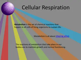
Physical activity requires energy; body gets energy through cellular
respiration; CO
2
is a byproduct.
1905 Haldane – experimentally identifies CO
2
as primary agent of
increasing ventilation.
1
As CO
2
builds in blood, reaction with H
2
O results in acidic product.
Receptors in brain detect acidity.
Signals sent to diaphragm to increase contraction rate.
Bio background & History (pt. 2)
1946 Gray – attempts to quantify this respiratory action by considering
“multiple factors”, (only one forcing term – CO
2
intake).
2
1967 Grodins – Considers a compartment model of flow of partial pressures
of CO
2
, through the body.
3
(This is what we’re going to discuss!)
Layout of Compartments
Subscript notation:
L = lungs
B = brain
T = soft tissue
i – into
o – out of
C = CO
2
concentration
f –
blood flow
Assumptions
Concentration out = Concentration
of compartment. (e.g. C
L,o
= C
L
)
Concentration entering brain and soft tissue is
delayed version of what left the lungs.
However, time delays = 0.
(e.g.
C
B,i
= C
L,o
)
Concentration leaving lungs is the same as
the concentration that enters.
Homogeneous (pt. 1 – example)
Using “rate-in – rate-out” method…
E.g. Brain
Since C
B,o
= C
B
and
C
B,i
= C
L,o
, we have (after converting
concentrations to partial pressure):
Homogeneous (pt. 2 - system)
Applying this method to all compartments, we have
Homgeneous (pt. 3 - solution)
Unique solution exists by Theorem 4.6.1, from McKibben
4
Non-homogeneous (pt. 1 - system)
Forcing terms
Partial pressures of brain, and soft
tissue.
Brain and soft tissue metabolic rates.
(could be indicative of “fitness” level)
Constant ventilation rate, based on
partial pressure leaving lungs. (not an
isolated system)
Non-homogeneous (pt. 2 - solution)
Unique solution exists by Theorem 5.3.1, from McKibben
4
Non-homogeneous (pt. 3 – graph)
Forcing vector = (5,5,0)
Forcing vector (0.01,0.01,0)
Semi-Linear (pt. 1 – system)
Changes: non-constant ventilation
rate; dependent on
•
Base ventilation rate.
•
Constant of rate increase.
•
CO
2
partial pressure in brain.
•
Threshold to CO
2
partial pressure.
Semi-Linear (pt. 2 – solution)
Unique “mild” solution exists by Theorem 7.6.1, from McKibben
4
Semi-Linear (pt. 3 – graphs)
Example solution plot
Example solution plot with ventilation
reduced by factor of 200.
Conclusion
Quantitatively, homogeneous case seems to model better.
Qualitatively, semi-linear case would be better since it takes more of
physical reality into account.
Further analysis of the terms of the system should provide evidence for the
latter.
References
[1] J. S. Haldane, and J. G. Priestley.
The Regulation of Lung-Ventilation.
The
Journal of Physiology, 32, 225–266. (1905).
[2] J. S. Gray.
The Multiple Factory Theory of the Control of Respiratory
Ventilation.
American Association for the Advancement of Science, 103, 739–
744, (1946).
[3] F. S. Grodins, J. Buell, A. Bart.
Mathematical analysis and digital simulation of
the respiratory control system.
J. Appl. Physiol., 22(2), 260–276, (1967).
[4] M. A. McKibben and M. D. Webster.
Differential Equations with MATLAB:
Exploration, Application, and Theory.
CRC Press. (2015).
[5] J. Keener and J. Sneyd.
Mathematical Physiology II: Systems Physiology.
Springer. (2009).
The End
(I can finally breathe!)
Explore the historical background and compartments of Grodins Pro Kumar's modeling of respiration, from differing breathing rates to the layout and assumptions of lungs, brain, and soft tissue. Learn how the homogeneous system is applied and the methods used to analyze this complex respiratory model.

Download Presentation

Please find below an Image/Link to download the presentation.
The content on the website is provided AS IS for your information and personal use only. It may not be sold, licensed, or shared on other websites without obtaining consent from the author. Download presentation by click this link. If you encounter any issues during the download, it is possible that the publisher has removed the file from their server.
E N D
Presentation Transcript
Modeling respiration with Grodins PRO KUMAR
Content Brief Bio I & History Compartments Assumptions (making life easier) Homogenous SGM-II Non-homogenous SGM-II Semi-Linear SGM-I Conclusion
Bio background & History (pt. 1) Differing breathing rates with differing activities. Why? Physical activity requires energy; body gets energy through cellular respiration; CO2 is a byproduct. 1905 Haldane experimentally identifies CO2 as primary agent of increasing ventilation.1 As CO2 builds in blood, reaction with H2O results in acidic product. Receptors in brain detect acidity. Signals sent to diaphragm to increase contraction rate.
Bio background & History (pt. 2) 1946 Gray attempts to quantify this respiratory action by considering multiple factors , (only one forcing term CO2intake).2 1967 Grodins Considers a compartment model of flow of partial pressures of CO2, through the body.3(This is what we re going to discuss!)
Layout of Compartments Lungs, CL,i CL,o Subscript notation: CL L = lungs f B = brain T = soft tissue fB Brain, i into CB CB,o CB,i o out of C = CO2 concentration f-fB f blood flow Soft tissue, CT CT,o CT,i
Assumptions Lungs, CL,i CL,o Concentration out = Concentration CL of compartment. (e.g. CL,o = CL ) Concentration entering brain and soft tissue is f delayed version of what left the lungs. fB Brain, However, time delays = 0. CB CB,o CB,i (e.g. CB,i = CL,o ) Concentration leaving lungs is the same as f-fB the concentration that enters. Soft tissue, CT CT,o CT,i
Homogeneous (pt. 1 example) Lungs, CL,i CL,o Using rate-in rate-out method CL f E.g. Brain ( ) dC t dt ( ) ( ) t = fB V f C C B Brain, , , B B B i B o CB,o CB,i CB f-fB Since CB,o = CB and CB,i = CL,o, we have (after converting concentrations to partial pressure): Soft tissue, CT CT,o CT,i ( ) dP t ( ) ( ) t = V K f K P P B dt , B co B co L o B 2 2
Homogeneous (pt. 2 - system) Lungs, CL,i CL,o Applying this method to all compartments, we have dP t V K CL ( ) f ( ) t = f K P B dt , B CO B CO L o 2 2 fB Brain, ( ) dP t CB,o CB,i CB ( ) ( ) t = V K K f f P T dt , T CO CO B L o f-fB 2 2 ( ) t dP Soft tissue, ( ) = , L o dt ( ) ( ) V K K f P t P t CT CT,o CT,i L CO CO B B T 2 2 = = ( ) ( ) P t P t P P P 0 0 B 0 ( ) t 1 P T = , 0 2 L o
Homgeneous (pt. 3 - solution) Unique solution exists by Theorem 4.6.1, from McKibben4 f B 0 0 V B f f ( ) B t t 0 0 0 V T ( ) ( ) ( ) t P t P t P P P P f f 0 B B B 0 V V = e L L 1 B , 2 L o
Non-homogeneous (pt. 1 - system) Forcing terms ( ) dP t ( ) ( ) t Partial pressures of brain, and soft tissue. = + V K M f K P P B dt , B co B B co L o B 2 2 Brain and soft tissue metabolic rates. (could be indicative of fitness level) ( ) dP t ( ) ( ) ( ) t = + V K M f f K P P T dt , T co T B co L o T 2 2 Constant ventilation rate, based on partial pressure leaving lungs. (not an isolated system) ( ) t dP ( ) = + , L o dt P P = ( ) t ( ) ( ) V K VK P K f P t P t , L co co L o co B B T 2 2 2 = = ( ) ( ) P t P t P 0 0 B 0 ( ) t 1 P T , 0 2 L o
Non-homogeneous (pt. 2 - solution) Unique solution exists by Theorem 5.3.1, from McKibben4 f f ( ) s 1 M K B B 0 0 0 0 V V f P B B f B f B B V f f ( ) ( ) B B t t t s 0 0 0 0 B CO 0 V V 2 T V T V ( ) ( ) ( ) t P t P t P P P P f f f f 0 B B B B B ( ) s 1 M K t V V V V V V = + ( ) e e f f TP ds T L L L L L L 1 B B V t 0 T CO 2 , 2 L o 0
Non-homogeneous (pt. 3 graph) Forcing vector = (5,5,0) Forcing vector (0.01,0.01,0)
Semi-Linear (pt. 1 system) ( ) dP t ( ) ( ) t = + V K M f K P P B dt Changes: non-constant ventilation rate; dependent on , B co B B co L o B 2 2 ( ) dP t ( ) ( ) ( ) t Base ventilation rate. = + V K M f f K P P T dt , T co T B co L o T 2 2 Constant of rate increase. ( ) t dP CO2 partial pressure in brain. Threshold to CO2 partial pressure. ( ) = + , L o dt V t P P = ( ) ( ) t ( ) ( ) V K V t P K f P t P t , L co L o co B B T 2 2 ( ) = + *[where ( ) ( ) ( ) T P t P max ( ) ] V k P t base B = = P t 0 0 B 0 ( ) t 1 P , 0 2 L o
Semi-Linear (pt. 2 solution) Unique mild solution exists by Theorem 7.6.1, from McKibben4 f f ( ) s 1 M K B B 0 0 0 0 f P V V B B f B f B B V f f ( ) ( ) B B t t t s 0 0 0 0 B CO 0 2 V V T T ( ) ( ) ( ) t P t P t P P P P f f f f 0 B B B B B ( ) s 1 M K 0 0 t V V V V = + ( ) e e f f P ds T L L L L 1 B B T V t 0 T CO 2 V t P , 2 L o ( ) , L o
Semi-Linear (pt. 3 graphs) Example solution plot with ventilation reduced by factor of 200. Example solution plot
Conclusion Quantitatively, homogeneous case seems to model better. Qualitatively, semi-linear case would be better since it takes more of physical reality into account. Further analysis of the terms of the system should provide evidence for the latter.
References [1] J. S. Haldane, and J. G. Priestley. The Regulation of Lung-Ventilation. The Journal of Physiology, 32, 225 266. (1905). [2] J. S. Gray. The Multiple Factory Theory of the Control of Respiratory Ventilation. American Association for the Advancement of Science, 103, 739 744, (1946). [3] F. S. Grodins, J. Buell, A. Bart. Mathematical analysis and digital simulation of the respiratory control system. J. Appl. Physiol., 22(2), 260 276, (1967). [4] M. A. McKibben and M. D. Webster. Differential Equations with MATLAB: Exploration, Application, and Theory. CRC Press. (2015). [5] J. Keener and J. Sneyd. Mathematical Physiology II: Systems Physiology. Springer. (2009).
The End (I can finally breathe!)


")
")


")
")
")
")
")
")
")
")
")