Factorial ANOVA: Understanding Experimental Design

Factorial ANOVA, Experimental Design, Analysis of Variance, Learning Outcomes, Research

• English

azurc Follow

Uploaded on Mar 04, 2025 | 0 Views

Download Presentation

Please find below an Image/Link to download the presentation.

The content on the website is provided AS IS for your information and personal use only. It may not be sold, licensed, or shared on other websites without obtaining consent from the author.If you encounter any issues during the download, it is possible that the publisher has removed the file from their server.

You are allowed to download the files provided on this website for personal or commercial use, subject to the condition that they are used lawfully. All files are the property of their respective owners.

The content on the website is provided AS IS for your information and personal use only. It may not be sold, licensed, or shared on other websites without obtaining consent from the author.

Presentation Transcript

1. Adapted from Jamison Fargo, PhD EDUC 6600 Slides Chapter 14 FACTORIAL ANOVA People can be divided into two classes: Those who go ahead and do something, and those who sit still and inquire, 'Why wasn't it done the other way? Oliver Wendell Holmes, American Physician, Writer, Humorist, HarvardProfessor, 1809-1894

2. People can be divided into two classes: Those who go ahead and do something, and those who sit still and inquire, 'Why wasn't it done the other way? Oliver Wendell Holmes, American Physician, Writer, Humorist, HarvardProfessor, 1809-1894

3. Dr. Petrov is interested in conducting an experiment where: 30 high school students are randomly assigned to a new computer simulation tool for learning geometry and 30 other students are randomly assigned to the standard lecture and paper/pencil problem solving format. However, Dr. Petrov is also interested in the effect of sex differences on learning outcomes. Adapted from: Jamison Fargo, PhD 3

4. ANALYSIS OF VARIANCE ANOVA types 1-Way ANOVA = 1 factor 2-Way ANOVA = 2 factors (focus of lecture) 3-Way ANOVA = 3 factors 4-Way ANOVA = 4 factors # levels of each factor determines ANOVA design # Levels: Row factor = 2, Column factor = 3 2-way ANOVA, 2X3 factorial design # Levels: Row factor = 4, Column factor = 3 2-way ANOVA, 4X3 factorial design 4

5. FACTORIAL 2-WAY ANOVA Simultaneously evaluate effect of 2 or more factors on continuous outcome Cross-classification Participants only belong to 1 mutually exclusive cell Within 1 level of row factor and 1 level of columns factor Typical 2-way ANOVA 3x2 design Row factor (A): 3 levels Column factor (B): 2 levels B B1 11 21 31 B2 12 22 32 A1 A2 A3 A 5

6. TEST OF ROW MAIN EFFECT Do row marginal means differ? Do population means differ across levels of row factor, averaging across levels of column factor? H0: j1 = j2 = jr H1: Not H0 B B1 M11 M21 M31 B2 M12 M22 M32 MB2 Marginals MA1 MA2 MA3 A1 A2 A3 A Marginals MB1 6

7. TEST OF ROW MAIN EFFECT Do column marginal means differ? Do population means differ across levels of column factor, averaging across levels of row factor? H0: j1 = j2 = jr H1: Not H0 B B1 M11 M21 M31 B2 M12 M22 M32 MB2 Marginals MA1 MA2 MA3 A1 A2 A3 A Marginals MB1 7

8. TEST OF INTERACTION EFFECT Does pattern of cell means differ? Are differences among population means across row factor similar across all levels of column factor (and vice versa)? H0:Differences among levels for 1 factor do not vary across levels of other factor H1: Not H0 B B1 M11 M21 M31 B2 M12 M22 M32 MB2 Marginals MA1 MA2 MA3 A1 A2 A3 A Marginals MB1 B B1 M11 M21 M31 B2 M12 M22 M32 MB2 Marginals MA1 MA2 MA3 A1 A2 A3 A Marginals MB1 8

9. POSSIBLE OUTCOMES 1. No significant main effects or interaction(s) 2. No significant interaction Significant main effect for rows, but not for columns Significant main effect for columns, but not for rows Significant main effects for both rows and columns 3. Significant interaction and Non-significant main effects for rows or columns Significant main effect for rows, but not for columns Significant main effect for columns, but not for rows Significant main effects for both rows and columns 9

10. REDUCED ERROR Adding factors that explain subject-to-subject variability in outcome reduces MSWand increases power Variance within (and thus across) individual cells is reduced as cases become more homogeneous in terms of their characteristics Subject-to-subject variability contributes to increased MSW = Less power Factors that do not have this effect may slightly decrease power dfW(which = N rc) decreases as # cells increases, increasing MSWand decreasing F-ratios Alternatives Restriction (subjects from 1-level only reduced generalizability) Repeated-measures (matched) designs 10

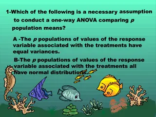
11. ASSUMPTIONS Similar to 1-Way ANOVA Independence Outcome is normally distributed in population Homogeneity of variance Variances within each cell are equal 11

12. VARIANCE COMPONENTS SSTotal partitioned into 4 components SSTotal = SS(R)ows + SS(C)olumns + SSRC + SSWithin When balanced, previous SSB from 1-Way ANOVA partitioned into 3 components: R, C, RC 1-way ANOVA uses groups and factorial ANOVA uses cells to compute SS Following equations are for balanced designs 12

13. SSR In computing row means all scores in a given row are averaged regardless of column nrow= # participants per row = + + ... ( + 2 2 2 [( ) ( ) ) ] SS n X X X X X X 1 2 R row row GM row GM row r GM 2 2 2 2 n n n n + + + ... X X X X 1 2 row row row r = = = = = 1 1 1 1 i i i i SS R n N row 13

14. SSC In computing column means all scores in a given column are averaged regardless of row ncol= # participants per column = + + ... ( + 2 2 2 [( ) ( ) ) ] SS column n X X X X X X 1 2 C col GM col GM col r GM 2 2 2 2 n n n n + + + ... X X X X 1 2 col col col r = = = = = 1 1 1 1 i i i i SS C n N col 14

15. SSRC Variability among cell means when variability due to individual row and column effects have been removed = + + ... ( + 2 2 2 [( ) ( ) ) ] SS n X X X X X X SS SS 11 12 RC cell cell GM cell GM cell rc GM R C 2 2 2 2 n n n n + + + ... X X X X 11 12 cell cell cell rc = = = = = 1 1 1 1 i i i i SS SS SS RC R C n N cell 15

16. SSW SS within each cell added together SSW = SS11 + SS12 + + SSrc For each cell, all scores within that cell are subtracted from cell mean, squared, and summed n rc ( ) rc 2 = SS X X W irc rc 1,1 = = 1 j i 2 2 2 n n n + + + ... X X X 11 12 cell cell cell rc n = = = = 1 1 1 i i i 2 i SS X W n = 1 i cell = SS SS SS SS SS W T R C RC 16

17. DEGREES OF FREEDOM dfTotal = NT - 1 Partitioned into 4 parts dfTotal = dfR + dfC +dfRC +dfW dfR = r 1 dfC = c 1 dfRC = (r 1)(c 1) dfW = (N rc) Assumes nare same for all cells Otherwise, (nrc 1): sum of n 1 per cell 17

18. VARIANCE ESTIMATES Obtain 4 variance estimates when each variance component is divided by its df MSR= Row variance estimate Sensitive to effects of factor A MSC= Column variance estimate Sensitive to effects of factor B MSRC= Row x Column variance estimate Sensitive to interaction effects of A and B MSW= Within-cells variance estimate Not sensitive to effects of any factor 18

19. F-STATISTICS Significance testing of 3 variance estimates Distinct Fstat for each MSR / MSWithin : Factor A MSC / MSWithin : Factor B MSRC / MSWithin : Interaction between factors A and B Each Fstat compared to distinct Fcrit Based on dfEffect(e.g., dfR)and dfWithin Reject H0: Fstat > Fcrit 19

20. SUMMARY TABLE SS df MS F p Source Row Column R x C Within X X Total X X X 20

21. INTERACTIONS Interaction between 2 factors: 2-way interaction 3 factors: 3-way interaction Quite rare, be skeptical Significance indicates that the effect of 1 factor is not same at all levels of another factor i.e. the effect of 1 factor depends on the level of the other Effect of variables combined is different than would be predicted by either variable alone Most interesting results, but more difficult to explain or interpret than main effects 21

22. INTERACTIONS Disordinal Direction or order of effects is reversed for different subgroups Ordinal Direction or order of effects is similar for different subgroups 6 100 Male Female M Phonemic Errors Mean Test Score 90 5 80 4 70 3 High SES Low SES 60 2 50 1 40 0 Control Treatment LTLE RTLE Study Group Hemisphere 22

23. INTERACTIONS Significance of interaction always evaluated 1st If significant, interpret interaction, not main effects If non-significant, interpret main effects Once we know effects of 1 factor are tempered by or contingent on levels of another factor (as in an interaction), interpretation of either factor (main effect) alone is problematic Best interpreted through visualization Cell means plot Interactions exist if lines cross or will cross (non- parallel) Design graph to best illustrate Outcome on y-axis Select factor for x-axis Other factor(s) represented by separate lines Selection guides interpretation, can dictate whether plot is ordinal/disordinal

24. INTERACTIONS Some recommend only interpreting significant main effects (Keppel & Wickens, 2004) When there is no significant interaction (Cautiously) when there is a significant interaction, but 1) interaction effect size is small relative to that of main effects and 2) there is an ordinal pattern to the means However, must report all main and interaction effects regardless of statistical significance 24

25. NEED FOR TESTING INTERACTIONS Results may be distorted if additional factors are not included in analysis so that interactions are not tested E.g., If experimental effects of a drug had opposite effects in men and women, the variable representing drug effects may appear to be ineffective (non-significant main effect) without including the variable for sex differences If interaction terms are non-significant, increased confidence that effect of key factor (e.g., drug treatment) is generalizable to all levels of other factors (e.g., sex) 25

26. EXAMPLE FROM TEXT Effect of sleep deprivation and compensating stimulation on performance of complex motor task Outcome: Video game score simulating driving truck at night Factor A (Row): Sleep deprivation 1. Control: Normal sleep schedule 2. Jet lag: Normal sleep amount, but during different hours 3. Interrupted: Normal sleep amount, but only for 2 hours at a time 4. Total Deprivation: No sleep for 4 days Factor B (Column): Stimulation conditions 1. Placebo: Told they are given a stimulant pill (really placebo) 2. Caffeine: Told they are given a stimulant pill (really stimulant) 3. Reward: Given mild electric shocks for mistakes and given a monetary reward for good performance 26

27. EXAMPLE H0 Deprivation control = jetlag = interrupted = deprive H0 Stimulus placebo = caffeine = reward H0 Interaction Effect of two factors is additive (no multiplicative or interaction effect) Effect of 1 factor does NOT depend on level of other factor 27

28. EXAMPLE Score Stimulus Stimulus Deprivation Deprivation 24 1 Placebo 20 1 Placebo 29 1 Placebo 20 1 Placebo 28 1 Placebo 22 1 Placebo 18 1 Placebo 16 1 Placebo 25 1 Placebo 27 1 Placebo 16 1 Placebo 20 1 Placebo 11 1 Placebo 19 1 Placebo 14 1 Placebo 14 1 Placebo 17 1 Placebo 12 1 Placebo 18 1 Placebo 10 1 Placebo 26 2 Caffeine 22 2 Caffeine 20 2 Caffeine 30 2 Caffeine 27 2 Caffeine 1 1 1 1 1 2 2 2 2 2 3 3 3 3 3 4 4 4 4 4 1 1 1 1 1 Control Control Control Control Control Jet Lag Jet Lag Jet Lag Jet Lag Jet Lag Interrupt Interrupt Interrupt Interrupt Interrupt Total Dep Total Dep Total Dep Total Dep Total Dep Control Control Control Control Control Stimulus Type Placebo 24 20 29 20 28 22 18 16 25 27 16 20 11 19 14 14 17 12 18 10 Caffeine 26 22 20 30 27 25 31 24 27 21 23 28 26 17 19 23 16 26 18 24 Reward 28 23 24 30 33 26 20 32 23 30 16 13 12 18 19 15 11 19 11 17 Control Depriviation Type Jet Lag Interrupt Total Deprivation

29. Proportion of variation in outcome accounted for by a particular factor or interaction term EFFECT SIZE Eta-squared ( 2) 1-way ANOVA SSBetween / SSTotal 2-way ANOVA Row factor: SSR / SSTotal Column factor: SSC / SSTotal Interaction: SSRC / SSTotal Interpretation: Range: 0 to 1 Small: .01 to .06 Medium: .06 to .14 Large: > .14 29

30. EFFECT SIZE 2 are biased parameter estimates Should estimate omega squared ( 2) Substitute SSand df values * SS df MS Effect SS Effect MS + Within = 2 Total Within Same interpretation as 2 30

31. EFFECT SIZE When all factors are experimental or when many factors are included in analysis, SS due to a factor or interaction will be small relative to SSTotal Partial effect size estimates are often reported Proportion of variation in outcome accounted for by a particular factor or interaction term, excluding other main effects or interaction sources of variation SS SS SS + Effect 2 Partial = Effect Within ( )/ ] + df MS MS N MS Effect MS Effect MS Within N = 2 Partial [ ( )/ df Effect Effect Within Within 31

32. MULTIPLE COMPARISONS Factorial ANOVA produces omnibus results No indication of specific level (group) differences within or across factor(s) Multiple comparisons elucidate differences within significant main effects or interactions Pattern of results dictates approach E.g., Significant main effects, but no interaction Each of the 3 F-tests in a 2-Way ANOVA represents a planned comparison No adjustment to EWnecessary However, within each main-effect and interaction a separate family of possible multiple comparisons may be conducted EWmust be controlled within each family 32

33. NON-SIGNIFICANT INTERACTION Evaluation of significant main effect(s) Factors with 2 levels No multiple comparisons required Factors with > 2 levels 2-way ANOVA is reduced to two 1-Way ANOVAs Simple (pairwise) or complex (linear) contrasts are computed within individual significant main-effect(s) (ignoring others) 33

34. NON-SIGNIFICANT INTERACTION Significant main-effects B B1 M11 M21 M31 B2 M12 M22 M32 MB2 Marginals MA1 MA2 MA3 A1 A2 A3 Simple or complex comparisons among marginal means (levels) A Marginals MB1 No further tests if F-test of main-effect indicates difference 34

35. EXAMPLE 1: NON-SIGNIFICANT INTERACTION Sleep deprivation, stimulant, and motor performance example Anova Table (Type II tests) Response: score Sum Sq Df F value Pr(>F) Deprivation 897.0 3 18.2406 4.896e-08 *** Stimulus 217.6 2 6.6385 0.002849 ** Interaction 194.8 6 1.9803 0.087003 . Residuals 786.8 48 Non-significant interaction Both main-effects are significant Need to compare marginal means for differences among levels 35

36. EXAMPLE 1: NON-SIGNIFICANT INTERACTION Motor Performance as a Function of Sleep and Stimuls Condition Motor Performance as a Function of Sleep and Stimuls Condition 30 30 Stimulus Placebo Stimulus Caffeine Stimulus Reward Performance Scores Performance Scores 25 Average 25 20 20 15 15 10 10 Control Jet Lag Interrupt Total 1 2 3 4 Deprivation Deprivation Type Deprivation Type Figure on left indicates main effect for deprivation type collapsing across levels of stimulant type Average of simple (main) effects Simple main effects are shown by the lines in figure on right When interaction is tested it is really a test of the H0that all simple effects are similar 36

37. EXAMPLE 1: NON-SIGNIFICANT INTERACTION Run 1-Way ANOVA on main-effects deemed significant in 2-Way ANOVA Optional Run multiple comparisons, controlling EW within each contrast Pairwise: Tukey, Bonferroni Linear contrasts: Contr.helmert 37

38. EXAMPLE 1: NON-SIGNIFICANT INTERACTION Conduct 1-Way ANOVA in R as before, select pairwise comparisons for Tukey tests Alternative by hand ; p-values close, not exactly the same TukeyHSD(aov_4_object$aov, "dep_F", ordered = F) TukeyHSD(aov_4_object$aov, "stim_F", ordered = F) plot(TukeyHSD(aov_4_object$aov, "dep_f")) plot(TukeyHSD(aov_4_object$aov, "stim_f")) 38

39. SIGNIFICANT INTERACTION Simple (main) effects of interaction are tested One factor is selected as stratifying factor Similar to deciding which factor to put on x-axis in means plot Let theory and research questions guide selection Levels (cells) of other factor are compared within each level of stratified factor Can redo analysis by reversing which factor is stratified and which is examined Comparing cell, rather than marginal, means 39

40. SIGNIFICANT INTERACTION Simple main effects generally tested within each level of stratifying factor 2-levels Simple, pairwise comparisons: Tukey HSD or t-tests with Bonferroni correction > 2 levels Modified 1-way ANOVA followed by simple or complex comparisons B B1 M11 M21 M31 B2 M12 M22 M32 MB2 Marginals MA1 MA2 MA3 A1 A2 A3 A Marginals MB1 B B1 M11 M21 M31 B2 M12 M22 M32 MB2 Marginals MA1 MA2 MA3 A1 A2 A3 A Marginals MB1 40

41. SIGNIFICANT INTERACTION Modified 1-Way ANOVA tests of simple main effects often done by hand Obtain MSBetween from standard 1-Way ANOVA Comparing means across 1 level of 1 factor within 1 level of another factor Obtain MSWithin from original 2-Way ANOVA Ensure homogeneity of variance assumption is reasonably satisfied MS MS (1-way ANOVA) Between = Simple Effect F (2-way ANOVA) ) from 1-way ANOVA Within df Within ( , Critical F df Between 41

42. UNBALANCED DESIGNS Equal ns in each cell = Orthogonal design Factors are independent/uncorrelated so that significance of any effect is independent of significance of other effects (including interaction) Most research consists of unbalanced data As ns across cells become more unequal, factors become more dependent/correlated Unbalanced: SSBetween SSR + SSC + SSRC More difficult to determine independent effects of each factor Previous equations and R commands will not work correctly for unbalanced designs 42

43. UNBALANCED DESIGNS Balanced Unbalanced F1 DV DV F1 F2 F2 F1xF2 F1xF2 Sum of areas where factors overlap with DV = SSB Remaining portion of DV = SSW Sum of areas where factors overlap with DV SSB Some areas counted twice Remaining portion of DV = SSW 43

44. 1. Equal cell sizes Factor A Factor B a1 a2 Row Marginal Means M = 125 n = 100 M = 225 n = 100 b1 M = 100 n = 50 M = 200 n = 50 M = 150 n = 100 M = 150 n = 50 M = 250 n = 50 M = 200 n = 100 b2 Column Marginal Means 2. Unequal cell sizes Factor A Factor B a1 a2 Row Marginal Means M = 145 n = 100 M = 205 n = 100 b1 M = 100 n = 10 M = 200 n = 90 M = 190 n = 100 M = 150 n = 90 M = 250 n = 10 M = 160 n = 100 b2 Column Marginal Means Individual cell means and marginal ns are the same across both tables. Main effects (marginal means) differ across tables as a function of different cell ns. Conclusions from ANOVA may vastly differ.

45. UNBALANCED DESIGNS Reason for unequal ns should be random, not related to factor(s) themselves (more difficult with non-experimental studies) If not so, validity of results is questionable when regular ANOVA procedures are employed Adjustments made to ANOVA to correct for unequal ns 1. Analysis of weighted means: Non-recommended, but common, approach where imbalance is slight and imbalance is random 1. Harmonic mean of cell ns is used in computation of various MS 2. Total N is adjusted = Harmonic mean of all cell sizes x # cells 3. MSWithin = Weighted average of cell variances 4. Each row and column mean computed = Simple (non-weighted) average of cell means in a given row or column 2. Alternate SS calculations to handle overlapping variation accounted for in outcome (Coming up next!) 3. Regression analysis (Take EDUC/PSY 7610!) # cells Harmonic mean = n 1 n = i 1 i 45

46. ALTERNATIVE SS CALCULATIONS Several methods for partitioning or allocating variation between outcome and factor(s) to account for unbalanced designs Commonly used Type I SS: Sequential or Hierarchical Type II SS: Partially Sequential Type III SS: Simultaneous or Regression Specialized and less commonly used Type IV SS: Don t use Type V SS: Used for fractional factorial designs Type VI SS: Effective hypothesis tests though sigma-restricted coding 46

47. ALTERNATIVE SS RECOMMENDATIONS Type II or III SS recommended in most cases Results should be fairly consistent Type III is most commonly used Nothing wrong with Type II Considered by some to be more powerful, especially when testing main effects Uncertainty of results when n are vastly unbalanced Not an issue when design is balanced Type I-III yield same results Even when unbalanced, interaction result same 47

48. INTERACTION CONTRASTS An alternative is to perform interaction contrasts , rather than immediately testing simple effects With a 2x2 design, only tests of simple main effects are possible With a 2x3 design, 3 separate 2x2 ANOVAs may be conducted Interaction magnitude (and significance) can differ from one subset to another Simple effects can be used following significant interaction subsets MSB for overall interaction = average of MSInteractionsfor separate interaction subsets 48

49. IGNORING FACTORIAL DESIGN Treat each cell as a separate group (e.g., M/Rep, M/Dem, F/Rep, F/Dem) and run analysis as 1-Way ANOVA with R*C groups? Results in same SSBetween as factorial design (SSR + SSC + SSRC ; when study is balanced) Cannot see patterns in data, as all levels of all factors are blended together in each group Cannot as easily observe interaction effects Limits identification of characteristics that uniquely differentiate participants More cumbersome when many factors included Less powerful 49

50. REPORTING RESULTS Marginal Ms for main effects, cell Ms for interactions and their SDs (or SEs) and CIs No need to report MSW For each significant effect F(dfEffect, dfWithin) = Fstat, p-value, effect size ( 2or 2) Results of post-hoc or planned comparisons Figures are *extremely* helpful! 50

Load More ...