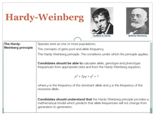
Equilibria in Populations: Hardy-Weinberg Principle
Exploring the concept of equilibria in populations, focusing on Hardy-Weinberg principles and its implications. The discussion covers allele distributions, genotype frequencies, maintenance of equilibrium across generations, and scenarios where equilibrium may be violated. Key points include basic principles, Hardy-Weinberg equilibrium conditions, implications of allele frequency stability, and real-world examples of genetic phenomena. The content emphasizes the importance of genetic equilibrium in understanding population genetics and evolutionary patterns.

Download Presentation

Please find below an Image/Link to download the presentation.
The content on the website is provided AS IS for your information and personal use only. It may not be sold, licensed, or shared on other websites without obtaining consent from the author.If you encounter any issues during the download, it is possible that the publisher has removed the file from their server.
You are allowed to download the files provided on this website for personal or commercial use, subject to the condition that they are used lawfully. All files are the property of their respective owners.
The content on the website is provided AS IS for your information and personal use only. It may not be sold, licensed, or shared on other websites without obtaining consent from the author.
E N D
Presentation Transcript
EQUILIBRIA IN POPULATIONS CSE280 Vineet Bafna
Basic Principles In a stable population, the distribution of alleles obeys certain laws Not really, and the deviations are interesting HW Equilibrium (due to mixing in a population) Linkage (dis)-equilibrium Due to recombination CSE280 Vineet Bafna
Hardy-Weinberg principle Time (generations) A Given: Population of diploid individuals and a locus with alleles, A & a 3 Genotypes: AA, Aa, aa Q: Will the frequency of alleles and genotypes remain constant from generation to generation? a
To the Editor of Science: I am reluctant to intrude in a discussion concerning matters of which I have no expert knowledge, and I should have expected the very simple point which I wish to make to have been familiar to biologists. However, some remarks of Mr. Udny Yule, to which Mr. R. C. Punnett has called my attention, suggest that it may still be worth making... . A little mathematics of the multiplication-table type is enough to show .the condition for this is q2 = pr. And since q12 = p1r1, whatever the values of p, q, and r may be, the distribution will in any case continue unchanged after the second generation
Hardy Weinberg equilibrium Suppose, Pr(A)=p, and Pr(a)=1-p=q If certain assumptions are met Large, diploid, population Discrete generations Random mating No selection, Then, in every generation Aa AA aa
Hardy-Weinberg principle Time (generations) In the next generation A a
Hardy Weinberg: Generalization Multiple alleles with frequencies By HW, q1,q2, ,qH Pr[homozygous genotype i]=qi Pr[heterozygous genotype i,j] =2qiqj 2 Multiple loci?
Hardy Weinberg: Implications The allele frequency does not change from generation to generation. True or false? It is observed that 1 in 10,000 caucasians have the disease phenylketonuria. The disease mutation(s) are all recessive. What fraction of the population carries the mutation? Males are 100 times more likely to have the red type of color blindness than females. Why? Individuals homozygous for S have the sickle-cell disease. In an experiment, the ratios A/A:A/S: S/S were 9365:2993:29. Is HWE violated? Is there a reason for this violation? A group of individuals was chosen in NYC. Would you be surprised if HWE was violated? Conclusion: While the HW assumptions are rarely satisfied, the principle is still important as a baseline assumption, and significant deviations are interesting. CSE280 Vineet Bafna
A modern example SNP-chips can give us the genotype at each site based on hybridization. Plot the 3 genotypes at each locus on 3 separate horizontal lines. 1/1 0/1 0/0 Genomic location 1 /1 0/1 Zoomed Out Picture 0/0 Genomic location
A modern example of HW application SNP-chips can give us the allelic value at each polymorphic site based on hybridization. What is peculiar in the picture? What is your conclusion?
The power of HWE Violation of HWE is common in nature Non-HWE implies that some assumption is violated Figuring out the violated assumption leads to biological insight
Linkage Equilibrium HW equilibrium is the equilibrium in allele frequencies at a single locus. Linkage equilibrium refers to the equilibrium between allele occurrences at two loci. LE is due to recombination events First, we will consider the case where no recombination occurs. L.E. H.W.E
Before you start, SNP matrix The infinite sites assumption Recombination Genealogy/phylogeny Basic data structures and algorithms
Reconstructing perfect phylogeny 12345678 01000000 00110110 00110100 00110000 00110000 10000000 10001000 10001001 2 7 6 3 4 5 1 8 We consider the directed (rooted) case. The root is all 0s, and all mutations are of the form 0 1
Columns 12345678 01000000 00110110 00110100 00110000 10000000 10001000 10001001 i A:0 B:1 C:1 D:1 E:0 F:0 G:0 CSE280 Vineet Bafna
Inclusion Property of Perfect Phylogeny For any pair of columns i,j, one of the following holds i1 j1 j1 i1 i1 j1 = For any pair of columns i,j i < j if and only if i1 j1 Note that if i<j then the edge containing i is an ancestor of the edge containing j i j CSE280 Vineet Bafna
Reconstruction of perfect phylogeny :12345678 A:01000000 B:00110110 C:00110100 D:00110000 E:10000000 F:10001000 G:10001001 CSE280 Vineet Bafna
Sort columns :12345678 A:01000000 B:00110110 C:00110100 D:00110000 E:10000000 F:10001000 G:10001001 3 0 1 1 1 0 0 0 7 0 1 0 0 0 0 0 4 0 1 1 1 0 0 0 6 0 1 1 0 0 0 0 2 1 0 0 0 0 0 0 1 0 0 0 0 1 1 1 8 0 0 0 0 0 0 1 5 0 0 0 0 0 1 1 A: B: C: D: E: F: G: CSE280 Vineet Bafna
Add First column 3 0 1 1 1 0 0 0 7 0 1 0 0 0 0 0 4 0 1 1 1 0 0 0 6 0 1 1 0 0 0 0 2 1 0 0 0 0 0 0 1 0 0 0 0 1 1 1 8 0 0 0 0 0 0 1 5 0 0 0 0 0 1 1 A: B: C: D: E: F: G:
Add First column 3 0 1 1 1 0 0 0 7 0 1 0 0 0 0 0 4 0 1 1 1 0 0 0 6 0 1 1 0 0 0 0 2 1 0 0 0 0 0 0 1 0 0 0 0 1 1 1 8 0 0 0 0 0 0 1 5 0 0 0 0 0 1 1 A: B: C: D: E: F: G:
Columns 3,4,5 3 0 1 1 1 0 0 0 7 0 1 0 0 0 0 0 4 0 1 1 1 0 0 0 6 0 1 1 0 0 0 0 2 1 0 0 0 0 0 0 1 0 0 0 0 1 1 1 8 0 0 0 0 0 0 1 5 0 0 0 0 0 1 1 A: B: C: D: E: F: G: A 2 B C D E F G
Columns 3 0 1 1 1 0 0 0 7 0 1 0 0 0 0 0 4 0 1 1 1 0 0 0 6 0 1 1 0 0 0 0 2 1 0 0 0 0 0 0 1 0 0 0 0 1 1 1 8 0 0 0 0 0 0 1 5 0 0 0 0 0 1 1 A: B: C: D: E: F: G: A 2 B C 6 3,4 D E F G
A perfect phylogeny 3 0 1 1 1 0 0 0 7 0 1 0 0 0 0 0 4 0 1 1 1 0 0 0 6 0 1 1 0 0 0 0 2 1 0 0 0 0 0 0 1 0 0 0 0 1 1 1 8 0 0 0 0 0 0 1 5 0 0 0 0 0 1 1 A 2 A: B: C: D: E: F: G: B 6 C 3,4 D 1 E F G 5 8
A perfect phylogeny 3 0 1 1 1 0 0 0 7 0 1 0 0 0 0 0 4 0 1 1 1 0 0 0 6 0 1 1 0 0 0 0 2 1 0 0 0 0 0 0 1 0 0 0 0 1 1 1 8 0 0 0 0 0 0 1 5 0 0 0 0 0 1 1 A 2 A: B: C: D: E: F: G: B 6 C 3,4 D 1 E F G 5 8
0s and 1s can be reversed 3 0 1 1 1 0 0 0 7 0 1 0 0 0 0 0 4 1 0 0 0 1 1 1 6 1 0 0 1 1 1 1 2 1 0 0 0 0 0 0 1 1 1 1 1 0 0 0 8 0 0 0 0 0 0 1 5 0 0 0 0 0 1 1 A 2 A: B: C: D: E: F: G: B 6 C 3,4 D 1 E F G 5 8
Unrooted case 4 0 1 1 1 0 0 0 3 0 1 1 1 0 0 0 7 0 1 0 0 0 0 0 4 1 0 0 0 1 1 1 6 1 0 0 1 1 1 1 2 1 0 0 0 0 0 0 1 1 1 1 1 0 0 0 8 0 0 0 0 0 0 1 5 0 0 0 0 0 1 1 Switch the values in each column, so that 0 is the majority element. Apply the algorithm for the rooted case. Relabel columns and individuals to the original values. A: B: C: D: E: F: G: CSE280 Vineet Bafna
Unrooted perfect phylogeny We transform matrix M to a 0-major matrix M0. if M0 has a directed perfect phylogeny, M has a perfect phylogeny. If M has a perfect phylogeny, does M0 have a directed perfect phylogeny?
Unrooted case Theorem: If M has a perfect phylogeny, there exists a relabeling, and a perfect phylogeny s.t. Root is all 0s For any SNP (column), #1s #0s All edges are mutated 0 1 CSE280 Vineet Bafna
Finding a center of an unrooted phylogeny Is it possible to find a node or an edge so that none of the children have more than n/2 nodes?
Proof Consider the perfect phylogeny of M. Find the center: Root at the center, and direct all mutations from 0 1 away from the root. QED If the theorem is correct, then simply relabeling all columns so that the majority element is 0 is sufficient. CSE280 Vineet Bafna
Homework Problems What if there is missing data? (An entry that can be 0 or 1)? What if recurrent mutations are allowed (infinite sites is violated)? CSE280 Vineet Bafna
Linkage Disequilibrium CSE280 Vineet Bafna
Quiz Recall that a SNP data-set is a binary matrix. Rows are individual (chromosomes) Columns are alleles at a specific locus Suppose you have 2 SNP datasets of a contiguous genomic region but no other information One from an African population, and one from a European Population. Can you tell which is which? How long does the genomic region have to be? CSE280 Vineet Bafna
Linkage (Dis)-equilibrium (LD) Consider sites A &B Case 1: No recombination Each new individual chromosome chooses a parent from the existing haplotype A B 0 1 0 1 0 0 0 0 1 0 1 0 1 0 1 0 1 0 CSE280 Vineet Bafna
Linkage (Dis)-equilibrium (LD) Consider sites A &B Case 2: diploidy and recombination Each new individual chooses a parent from the existing alleles A B 0 1 0 1 0 0 0 0 1 0 1 0 1 0 1 0 1 1 CSE280 Vineet Bafna
Linkage (Dis)-equilibrium (LD) Consider sites A &B Case 1: No recombination Each new individual chooses a parent from the existing haplotype Pr[A,B=0,1] = 0.25 Linkage disequilibrium Case 2: Extensive recombination Each new individual simply chooses and allele from either site Pr[A,B=(0,1)]=0.125 Linkage equilibrium A B 0 1 0 1 0 0 0 0 1 0 1 0 1 0 1 0 CSE280 Vineet Bafna
LD In the absence of recombination, Correlation between columns The joint probability Pr[A=a,B=b] is different from P(a)P(b) With extensive recombination Pr(a,b)=P(a)P(b) CSE280 Vineet Bafna
Measures of LD Consider two bi-allelic sites with alleles marked with 0 and 1 Define P00 = Pr[Allele 0 in locus 1, and 0 in locus 2] P0* = Pr[Allele 0 in locus 1] Linkage equilibrium if P00 = P0* P*0 The D-measure of LD D = (P00 - P0* P*0) = -(P01 - P0* P*1) = CSE280 Vineet Bafna
Other measures of LD D is obtained by dividing D by the largest possible value Suppose D = (P00 - P0* P*0) >0. Then the maximum value of Dmax= min{P0* P*1, P1* P*0} If D<0, then maximum value is max{-P0* P*0, -P1* P*1} D = D/ Dmax 0 1 -D D 0 Site 1 -D D 1 Site 2 CSE280 Vineet Bafna
Other measures of LD D is obtained by dividing D by the largest possible value Ex: D = abs(P11- P1* P*1)/ Dmax = D/(P1* P0* P*1 P*0)1/2 Let N be the number of individuals Show that 2N is the 2 statistic between the two sites 0 1 P00N 0 P0*N Site 1 1 Site 2 CSE280 Vineet Bafna
Digression: The 2test 0 1 O1 O2 0 O3 O4 1 ( ) 2 Oi- Ei i The statistic distribution (sum of squares of normal variables). A p-value can be computed directly behaves like a 2 Ei
Observed and expected 0 1 0 1 0 P01N P0*P*1N P00N P0*P*0N Site 1 1 P10N P11N P1*P*0N P1*P*1N = D/(P1* P0* P*1 P*0)1/2 Verify that 2N is the 2 statistic between the two sites
LD over time and distance The number of recombination events between two sites, can be assumed to be Poisson distributed. Let r denote the recombination rate between two adjacent sites r = # crossovers per bp per generation The recombination rate between two sites l apart is rl
LD over time Decay in LD Let D(t) = LD at time t between two sites r =lr P(t)00 = (1-r ) P(t-1)00 + r P(t-1)0* P(t-1)*0 D(t) =P(t)00 - P(t)0* P(t)*0 = P(t)00 - P(t-1)0* P(t-1)*0 (Why?) D(t) =(1-r ) D(t-1) =(1-r )t D(0) CSE280 Vineet Bafna
LD over distance Assumption Recombination rate increases linearly with distance and time LD decays exponentially. The assumption is reasonable, but recombination rates vary from region to region, adding to complexity This simple fact is the basis of disease association mapping. CSE280 Vineet Bafna
LD and disease mapping Consider a mutation that is causal for a disease. The goal of disease gene mapping is to discover which gene (locus) carries the mutation. Consider every polymorphism, and check: There might be too many polymorphisms Multiple mutations (even at a single locus) that lead to the same disease Instead, consider a dense sample of polymorphisms that span the genome CSE280 Vineet Bafna


 lineage is a tree")
 lineage is a tree")


-equilibrium (LD)")
-equilibrium (LD)")
-equilibrium (LD)")