Effective Data Handling and Feature Reduction Strategies

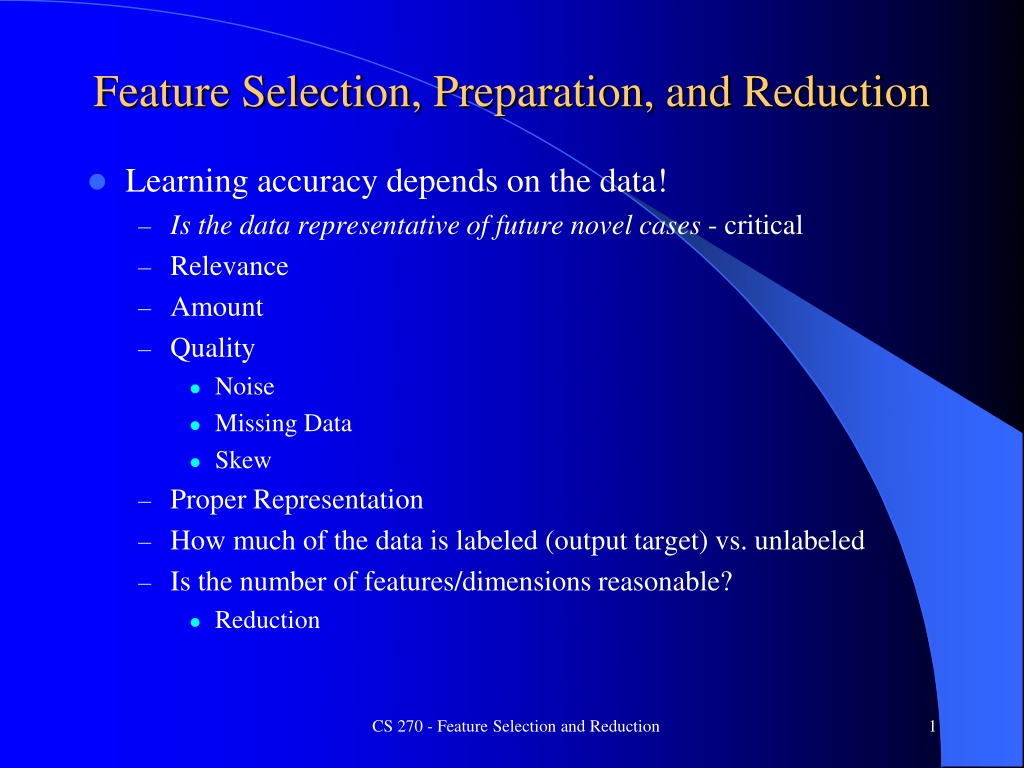
Feature Selection, Preparation, and Reduction Learning accuracy depends on the data! Is the data representative of future novel cases - critical Relevance Amount Quality Noise Missing Data Skew Proper Representation How much of the data is labeled (output target) vs. unlabeled Is the number of features/dimensions reasonable? Reduction CS 270 - Feature Selection and Reduction 1

Gathering Data Consider the task What kind of features could help Data availability Significant diversity in cost of gathering different features More the better (in terms of number of instances, not necessarily in terms of number of dimensions/features) The more features you have the more data you need Data augmentation, Jitter Increased data can help with overfit handle with care! Labeled data is best If not labeled Could set up studies/experts to obtain labeled data Use unsupervised and semi-supervised techniques Clustering Active Learning, Bootstrapping, Oracle Learning, etc. CS 270 - Feature Selection and Reduction 2

When to Gather More Data When trying to improve performance, you may need More Data Better Input Features Different Machine learning models or hyperparameters Etc. One way to decide if you need more/better data Compare your accuracy on training and test set If bad training set accuracy then you might need better data/ features. Though you might need a different learning model/hyperparameters If test set accuracy is much worse than training set accuracy then gathering more data is usually a good direction and consider better overfit avoidance. Learning model/hyperparameters could still be a significant issue. CS 270 - Feature Selection and Reduction 3

Data Representation Categorical/Symbolic Nominal No natural ordering Ordered/Ordinal Special cases: Time/Date, Addresses, Names, IDs, etc. Already discussed how to transform categorical to continuous data for models (e.g. perceptrons) which want continuous inputs Continuous Some models are better equipped to handle nominal/ordered data How to transform continuous to ordinal CS 270 - Feature Selection and Reduction 4

Transforming Continuous to Ordered Data Basic approach is to discretize/bin the continuous data How many bins differs by problem, enough to appropriately divide data Equal-Width Binning Bins of fixed ranges Does not handle skew/outliers well Equal-Height Binning Bins with equal number of instances Uniform distribution, can help for skew and outliers More likely to have breaks in high data concentrations Clustering More accurate, though more complex Bin borders can be an issue CS 270 - Feature Selection and Reduction 5

Supervised Binning The previous binning approaches do not consider the classification of each instance and thus they are unsupervised (Class-aware vs. Class-blind) Could use a supervised approach which attempts to bin such that learning algorithms may more easily classify Supervised approaches can find bins while also maximizing correlation between output classes and values in each bin Often rely on information theoretic techniques CS 270 - Feature Selection and Reduction 6

Data Normalization Normalization for continuous values (0-1 common) What if data has skew, outliers, etc. Standardization (z-score) Transform the data by subtracting the average and then dividing by the standard deviation allows more information on spread/outliers Look at the data to make these and other decisions! May be better served with a non-linear normalization based on the data spread CS 270 - Feature Selection and Reduction 7

Output Class Skew Nuclear reactor data Meltdowns vs. non-meltdowns If occurrence of certain output classes are rare Machine learners often just learn to output the majority class output value Most accurate southern California weather forecast Approaches to deal with Skew Undersampling: if 100,000 instances and only 1,000 of the minority class, keep all 1,000 of the minority class, and drop majority class examples until reaching a reasonable distribution but lose data Oversampling: Make duplicates of every minority instance and add it to the data set until reaching a reasonable distribution (Overfit possibilities) Could add new copies with jitter (be careful!) Have learning algorithm weight the minority class higher, or class with higher misclassification cost (even if balanced), learning rate, etc. Use Precision/Recall or ROC rather than just accuracy CS 270 - Feature Selection and Reduction 8

Transformed/Derived Variables (Meta-Features) Transform initial data features into better ones - Quadric machine was one example Transforms of individual variables Use area code rather than full phone number Determine the vehicle make from a VIN (vehicle id no.) Combining/deriving variables Height/weight ratio Difference of two dates Do some derived variables in your group project especially if features mostly given! Features based on other instances in the set e.g. This instance is in the top quartile of price/quality tradeoff Transforming/Deriving features requires creativity and some knowledge of the task domain but can be very effective in improving accuracy CS 270 - Feature Selection and Reduction 9

Relevant Data Typically do not use features where Almost all instance have the same value (no information) If there is a significant, though small, percentage of other values, then might still be useful Nominal feature where almost all instances have unique values (SSN, phone-numbers) Might be able to use a variation of the feature (such as area code) The feature is highly correlated with another feature In this case the feature may be redundant and only one is needed CS 270 - Feature Selection and Reduction 10

Missing Data BP Pain Out .5 Low 0 Need to consider approach for learning and execution (could differ) Throw out data with missing attributes Do only if rare, else could lose a significant amount of training set Doesn t work during execution Set (impute/imputation) attribute to its mode/mean (based on rest of data set) Too big of an assumption? Use a learning scheme (NN, DT, etc) to impute missing values Train imputing models with a training set which has the missing attribute as the target and the rest of the attributes as input features. Better accuracy, though more time consuming - multiple missing values? Impute based on the most similar instance(s) in the data set - SK KNNImputer Train multiple reduced input models without common missing features *Let unknown be just another attribute value Can work well in many cases Missing attribute may contain important information, (didn t vote can mean something about congressperson, extreme measurements aren t captured, etc.). Natural for nominal data With continuous data, can use an indicator node, or a value which does not occur in the normal data (-1, outside range, etc.), however, in the latter case, the model will treat this as an extreme ordered feature value and may cause difficulties .8 Hi 1 ? Low 1 1 ? 0 CS 270 - Feature Selection and Reduction 11

*Challenge Question* - Missing Data Given the dataset to the right, what approach would you use to deal with the two unknown values and what would those values be set to? Assume you are learning with an MLP and Backpropagation Throwing out those instances is not an option in this case I left out targets on purpose since they won t be available with novel data If your approach requires any modifications to the MLP inputs, be ready to explain exactly what those are x y z Out .1 .6 B .6 .6 G .3 .35 R .6 .45 G .6 .4 ? .8 ? B CS 270 - Feature Selection and Reduction 12

Dirty Data and Data Cleaning Dealing with bad data, inconsistencies, and outliers Many ways errors are introduced Measurement Noise/Outliers Poor Data Entry User lack of interest Most common birthday when B-day mandatory: November 11, 1911 Data collectors don't want blanks in data warehousing so they may fill in (impute) arbitrary values Data Cleaning Data analysis to discover inconsistencies Consider distribution of a feature s values (find mistakes/outliers) Clustering/Binning can sometimes help Noise/Outlier removal Requires care to know when it is noise and how to deal with this during execution Our experiments show hard instance removal (those always wrong, noise or not) during training increases subsequent accuracy CS 270 - Feature Selection and Reduction 13

Labeled and Unlabeled Data Accurately labeled data is always best Often there is lots of cheaply available unlabeled data which is expensive/difficult to label internet data, etc. Semi-Supervised Learning Can sometimes augment a small set of labeled data with lots of unlabeled data to gain improvements Bootstrapping: Iteratively use current labeled data to train model, use the trained model to label the unlabeled data, then train again including most confident newly labeled data, and re-label, etc., until some convergence Active Learning Out of a collection of unlabeled data, ML model queries for the next most informative instance to label Combinations of above and other techniques being proposed CS 270 - Feature Selection and Reduction 14

Semi-Supervised Learning Examples Combine labeled and unlabeled data with assumptions about typical data to find better solutions than just using the labeled data CS 270 - Feature Selection and Reduction 15

Active Learning Often query: 1) A low confidence instance (i.e. near a decision boundary) 2) An instance which is in a relatively dense neighborhood CS 270 - Feature Selection and Reduction 16

Active Learning Often query: 1) A low confidence instance (i.e. near a decision boundary) 2) An instance which is in a relatively dense neighborhood CS 270 - Feature Selection and Reduction 17

Active Learning Often query: 1) A low confidence instance (i.e. near a decision boundary) 2) An instance which is in a relatively dense neighborhood CS 270 - Feature Selection and Reduction 18

Your Project Proposals See description in Learning Suite Remember your example instance! Examples Look at Irvine Data Set, Kaggle, or OpenML to get a feel of what data sets look like Stick with supervised classification problems for the most part for the project proposals Tasks which interest you Too hard vs Too Easy Data should be able to be gathered in a relatively short time And, want you to have to battle with the data/features a bit. You can t just use a pretty much ready to go data set that you find! CS 270 - Feature Selection and Reduction 19

Feature Selection and Feature Reduction Given n original features, it is often advantageous to reduce this to a smaller set of features for actual training Can improve/maintain accuracy if we can preserve the most relevant information while discarding the most irrelevant information And/or can make the learning process more computationally and algorithmically manageable by working with less features Curse of dimensionality requires an exponential increase in data set size in relation to the number of features to learn without overfit thus decreasing features can be critical Feature Selection seeks a subset of the n original features which retains most of the relevant information Filters, Wrappers Feature Reduction combines/fuses the n original features into a smaller set of newly created features which hopefully retains most of the relevant information from all the original features - Data fusion (e.g. LDA, PCA, etc.) CS 270 - Feature Selection and Reduction 20

Feature Selection - Filters Given n original features, how do you select size of subset User can preselect a size p (< n) not usually as effective Usually try to find the smallest size where adding more features does not yield improvement Filters work independent of any particular learning algorithm Filters seek a subset of features which maximize some type of between class separability or other merit score Can score each feature independently and keep best subset e.g. 1st order correlation with output, fast, less optimal Can score subsets of features together Exponential number of subsets requires a more efficient, sub-optimal search approach How to score features is independent of the ML model to be trained on and is an important research area Decision Tree or other ML model pre-process CS 270 - Feature Selection and Reduction 21

Feature Selection - Wrappers Optimizes for a specific learning algorithm The feature subset selection algorithm is a "wrapper" around the learning algorithm 1. Pick a feature subset and pass it to learning algorithm 2. Create training/test set based on the feature subset 3. Train the learning algorithm with the training set 4. Find accuracy (objective) with validation set 5. Repeat for all feature subsets and pick the feature subset which gives the highest predictive accuracy (or other objective) Basic approach is simple Variations are based on how to select the feature subsets, since there are an exponential number of subsets CS 270 - Feature Selection and Reduction 22

Feature Selection - Wrappers Exhaustive Search - Exhausting Forward Search O(n2 learning/testing time) - Greedy 1. Score each feature by itself and add the best feature to the initially empty set FS (FS will be our final Feature Set) 2. Try each subset consisting of the current FS plus one remaining feature and add the best feature to FS 3. Continue until stop getting significant improvement (over a window) Backward Search O(n2 learning/testing time) - Greedy 1. Score the initial complete FS 2. Try each subset consisting of the current FS minus one feature in FS and drop the feature from FS causing least decrease in accuracy 3. Continue until dropping any feature causes a significant decreases in accuracy Branch and Bound and other heuristic approaches available CS 270 - Feature Selection and Reduction 23

PCA Principal Components Analysis PCA is one of the most common feature reduction techniques A linear method for dimensionality reduction Allows us to combine much of the information contained in n features into p features where p < n PCA is unsupervised in that it does not consider the output class/value of an instance There are other algorithms which do (e.g. LDA - Linear Discriminant Analysis) PCA works well in many cases where data features have mostly linear correlations Non-linear dimensionality reduction is also a successful area and can give better results for data with significant non-linear correlations between the data features CS 270 - Feature Selection and Reduction 24

PCA Overview Seek new set of bases which correspond to the highest variance in the data Transform n-dimensional normalized data to a new n- dimensional basis The new dimension with the most variance is the first principal component The next is the second principal component, etc. Note z1 combines/fuses significant information from both x1 and x2 Can drop dimensions for which there is little variance CS 270 - Feature Selection and Reduction 25

Variance and Covariance Variance is a measure of data spread in one feature/dimension n features, m instances in data set Note n in variance/covariance equations is number of instances in the data set, apologies Covariance measures how two dimensions (features) vary with respect to each other Normalize data features so they have similar magnitudes else covariance may not be as informative n ( ) ( ) Xi- X ( ( i=1 Xi- X ) )Yi-Y n -1 ) var(X) = i=1 n -1 n ( ) Xi- X ( cov(X,Y) = CS 270 - Feature Selection and Reduction 26

Covariance and the Covariance Matrix Considering the sign (rather than exact value) of covariance: Positive value means that as one feature increases or decreases the other does also (positively correlated) Negative value means that as one feature increases the other decreases and vice versa (negatively correlated) A value close to zero means the features are independent If highly covariant, are both features necessary? Covariance matrix is an n n matrix containing the covariance values for all pairs of features in a data set with n features (dimensions) The diagonal contains the covariance of a feature with itself which is the variance (i.e. the square of the standard deviation) The matrix is symmetric CS 270 - Feature Selection and Reduction 27

PCA Example First step is to center the original data around 0 by subtracting the mean in each dimension normalize first if needed Data x y x' y' 2.5 0.5 2.2 1.9 3.1 2.3 2.0 1.0 1.5 1.2 1.82 2.4 0.7 2.9 2.2 3.0 2.7 1.6 1.1 1.6 0.9 1.91 0.68 -1.32 0.38 0.08 1.28 0.48 0.18 -0.82 -0.32 -0.62 0 0.49 -1.21 0.99 0.29 1.09 0.79 -0.31 -0.81 -0.31 -1.01 0 Mean CS 270 - Feature Selection and Reduction 28

PCA Example Second: Calculate the covariance matrix of the centered data Only 2 2 for this case n Data x y x' y' ( )Yi-Y n -1 ) ( ) Xi- X ( 2.5 0.5 2.2 1.9 3.1 2.3 2.0 1.0 1.5 1.2 1.82 2.4 0.7 2.9 2.2 3.0 2.7 1.6 1.1 1.6 0.9 1.91 0.68 -1.32 0.38 0.08 1.28 0.48 0.18 -0.82 -0.32 -0.62 0 0.49 -1.21 0.99 0.29 1.09 0.79 cov(X,Y) = i=1 Covariance Matrix -0.31 -0.81 -0.31 -1.01 0 0.60177778 0.60422222 0.71655556 Mean CS 270 - Feature Selection and Reduction 29

PCA Example Third: Calculate the unit eigenvectors and eigenvalues of the covariance matrix (remember your linear algebra) Covariance matrix is always square n n and positive semi-definite, thus n non-negative eigenvalues will exist All eigenvectors (principal components) are orthogonal to each other and form the new set of bases/dimensions for the data (columns) The magnitude of each eigenvalue corresponds to the variance along each new dimension Just what we wanted! We can sort the principal components according to their eigenvalues Just keep those dimensions with the largest eigenvalues Principal Component 1 2 Eigenvalues Eigenvectors 1.26610816 -0.67284685, -0.7397818 0.05222517 -0.7397818, 0.67284685 CS 270 - Feature Selection and Reduction 30

PCA Example Below are the two eigenvectors overlaying the centered data Which eigenvector has the largest eigenvalue? Fourth Step: Just keep the p eigenvectors with the largest eigenvalues Do lose some information, but if we just drop dimensions with small eigenvalues then we lose only a little information, hopefully noise We can then have p input features rather than n The p features contain the most pertinent combined information from all n original features How many dimensions p should we keep? PC Eigenvalues Eigenvectors 1 1.26610816 -0.67284685, -0.7397818 2 0.05222517 -0.7397818, 0.67284685 1.226/(1.226+.052) = .96 Proportion of Variance Eigenvalue 1 2 3 4 5 6 7 n 31

PCA Example Last Step: Transform the n features to the p (< n) chosen bases (Eigenvectors) Transform data (m instances) with a matrix multiply T = A B A is a p n matrix with the p principal components in the rows, component one on top B is a n m matrix containing the transposed centered original data set TT is a m p matrix containing the transformed data set Now we have the new transformed data set with p features Keep matrix A to transform future centered data instances Below is the transform of both dimensions. Would if we just kept the 1st component for this case? 32

PCA Algorithm Summary Center the n normalized TS features (subtract the n means) Calculate the covariance matrix of the centered TS Calculate the unit eigenvectors and eigenvalues of the covariance matrix Keep the p (< n) eigenvectors with the largest eigenvalues 5. Matrix multiply the p eigenvectors with the centered TS to get a new TS with only p features 1. 2. 3. 4. Given a novel instance during execution 1. Center the normalized instance (subtract the n means) 2. Do the matrix multiply (step 5 above) to change the new instance from n to p features CS 270 - Feature Selection and Reduction 33

Terms PCA Homework 5 Number of instances in data set m 2 Number of input features n 1 Final number of principal components chosen p Use PCA on the given data set to get a transformed data set with just one feature (the first principal component (PC)). Show your work along the way. Show what % of the total information is contained in the 1st PC. Do not use a PCA package to do it. You need to go through the steps yourself, or program it yourself. You may use a spreadsheet, Matlab, etc. to do the arithmetic for you. You may use Python or any web tool to calculate the eigenvectors/eigenvalues from the covariance matrix. Optional: After, use any PCA solver (e.g. sklearn) and use it to solve the problem and check your answers. Original Data x y Out m1 .2 -.3 - m2 -1.1 2 - m3 1 -2.2 - m4 .5 -1 - m5 -.6 1 - mean CS 270 - Feature Selection and Reduction 34

PCA Summary PCA is a linear transformation, so if the features have highly non-linear correlations, the transformed data will be less useful Non linear dimensionality reduction techniques can sometimes handle these situations better (e.g. LLE, Isomap, Manifold-Sculpting) PCA is good at removing redundant linearly correlated features With high dimensional data the eigenvector is a hyper-plane Interesting note: The 1st principal component is the multiple regression plane that delta rule will always discover Caution: Not a "cure all" and can lose important info in some cases How would you know if it is effective? Just compare accuracies of original vs transformed data set CS 270 - Feature Selection and Reduction 35

Practical Feature Reduction Assume you have a data set with 50 features You might like to reduce if possible (you might hope for 10 or so, but let the results decide) Could try PCA Compare PCA with original training results to see how effective PCA is for the particular data set Could also try a wrapper (e.g. backward greedy) and compare its results and then go with what gives the best accuracy PCA Pro: Potentially fuses most information from all features into a new smaller set of features Con: Will fail if features have lots of non-linear correlations Wrappers Pro: Can handle data features with arbitrary non-linear correlations Con: Does not fuse info, those features which are dropped are completely gone CS 270 - Feature Selection and Reduction 36

Group Projects and Teams CS 270 - Feature Selection and Reduction 37