Dynamic Systems Analysis for Control Engineering
Explore the construction of system models, solving system equations, standard systems, system performance, and automatic control in the field of dynamic systems analysis. Understand topics like input excitation, impulse distribution, sinusoidal systems, transfer functions, block diagrams, and frequency response plotting.

Download Presentation

Please find below an Image/Link to download the presentation.
The content on the website is provided AS IS for your information and personal use only. It may not be sold, licensed, or shared on other websites without obtaining consent from the author. If you encounter any issues during the download, it is possible that the publisher has removed the file from their server.
You are allowed to download the files provided on this website for personal or commercial use, subject to the condition that they are used lawfully. All files are the property of their respective owners.
The content on the website is provided AS IS for your information and personal use only. It may not be sold, licensed, or shared on other websites without obtaining consent from the author.
E N D
Presentation Transcript
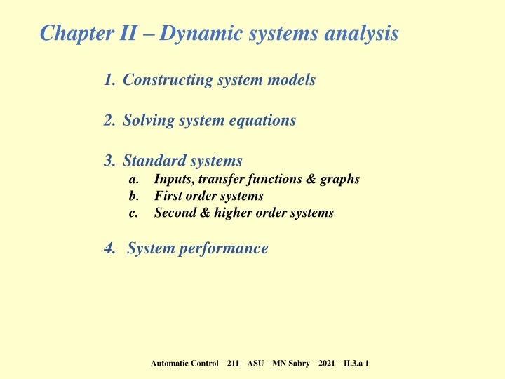
Chapter II Dynamic systems analysis 1. Constructing system models 2. Solving system equations 3. Standard systems a. Inputs, transfer functions & graphs b. First order systems c. Second & higher order systems 4. System performance Automatic Control 211 ASU MN Sabry 2021 II.3.a 1
Input excitations: A- Step & Ramp inputs Step Input (Ideal) t=0 1 0 0 0 t t ( ) ( ) t = = u t t Ramp Input 1 In reality ( ) u t 0.8 ( ) 0.5 tan + t a 1 0.6 t 0.4 0.2 0 -1 -0.75 -0.5 -0.25 a = 0.1 0 0.25 0.5 a = 0.01 0.75 1 a = 0.05 Automatic Control 211 ASU MN Sabry 2021 II.3.a 2
B- Impulse (Dirac distribution) dV dt = ( ) ( ) ( ) t = = = ; : u t I C if V t Ideally: No resistance t=0 Input I (Ideal) I 0 2 t ( ) ( ) t = + 1 2, 2 0 u t t t 0 2 t x(t) 0 t ( ) t dt = 1 In reality k 0 t m + a ( ) 30 u t c 2 2 a t 20 Point force t~ Q~10/ 10 10L 0 -0.25 -0.15 a = 0.1 -0.05 0.05 0.15 a = 0.01 0.25 Area~ P~F/Area(= ) a = 0.05 Automatic Control 211 ASU MN Sabry 2021 II.3.a 3
C- Sinusoidal Permanent magnet y(t) k LTI system m ~ Input: Output: Wait until steady state A ej( t+ ) c Electro magnet ej t=cos t+jsin t sin or cos does not matter Amplitude = 1 1 u(t) y(t) 0.5 A 0 Since LTI, @ steady state: - Output is sinusoidal - Output frequency = Input freq. A = A( ) = ( ) 0 2 4 6 8 10 -0.5 - -1 Automatic Control 211 ASU MN Sabry 2021 II.3.a 4
Transfer function, block diagram x(t) k f(t) Consider the system: m c ( ) ( ) ( ) ( ) + + = 2 2 md x t dt cdx t dt k x t f t ODE: ( ) ( ) X s F s 1 ( ) = = Taking the Laplace transform: G s + + 2 ms cs k Block diagram: Y(s) U(s) Input Output G(s) Output does NOT affect input Transfer function Automatic Control 211 ASU MN Sabry 2021 II.3.a 5
Block diagram G1 . G2 c=G2b b=G1a f=c d a a G1 G2 + G1 . G2 G3 a d=G3a G3 E = R F C = E G F = H C C Eliminate E E R Eliminate F + G ( ) ( ) R s ( ) ( ) G s H s F C s G s = H ( ) + 1 Automatic Control 211 ASU MN Sabry 2021 II.3.a 6
To plot frequency response: Bode plot Bode plot: Amplitude vs frequency 20 log10 G (decibel) -10 1 in dB ( ) = G s -20 + + 2 ms cs k -30 1 ( ) -40 = G j + 2 k m j c -50 log10 = + Re Im j -60 -1 -0.5 0 0.5 1 1.5 Im Bode plot: Phase vs frequency = G 0 -30 -60 -90 -120 Re -150 log10 -180 -1 -0.5 0 0.5 1 1.5 Automatic Control 211 ASU MN Sabry 2021 II.3.a 7
Polar plot 1 ( ) = G j + 2 k m j c Im = + Re Im j Re 0 = = -0.04 -0.02 0 0.02 0.04 0.06 0.08 -0.02 -0.04 = = -0.06 -0.08 = -0.1 Automatic Control 211 ASU MN Sabry 2021 II.3.a 8


")