Data Mining Anomaly/Outlier Detection

Data Mining
Anomaly/Outlier Detection
Lecture Notes for Chapter 9 (10 first Edition)
Introduction to Data Mining 2
nd
Edition
by
Tan, Steinbach,
Karpatne,
Kumar
New slides have been added and the original slides have
been significantly modified by
Christoph F. Eick


Lecture Organization COSC 3337
Anomaly/Outlier Detection
1.
Graphic-based Approaches
2.
Model-based
3.
One-Class SVM Approach
only briefly covered
4.
Distance-Based Approaches
5.
Reconstuction Error-based approach
0. Anomaly/Outlier Detection
l
What are anomalies/outliers?
–
The set of data points that are considerably different than the
remainder of the data
l
Variants of Anomaly/Outlier Detection Problems
–
G
i
v
e
n
a
d
a
t
a
b
a
s
e
D
,
f
i
n
d
a
l
l
t
h
e
d
a
t
a
p
o
i
n
t
s
x
D
w
i
t
h
a
n
o
m
a
l
y
s
c
o
r
e
s
g
r
e
a
t
e
r
t
h
a
n
s
o
m
e
t
h
r
e
s
h
o
l
d
t
–
G
i
v
e
n
a
d
a
t
a
b
a
s
e
D
,
f
i
n
d
a
l
l
t
h
e
d
a
t
a
p
o
i
n
t
s
x
D
h
a
v
i
n
g
t
h
e
t
o
p
-
n
l
a
r
g
e
s
t
a
n
o
m
a
l
y
s
c
o
r
e
s
f
(
x
)
–
G
i
v
e
n
a
d
a
t
a
b
a
s
e
D
,
c
o
n
t
a
i
n
i
n
g
m
o
s
t
l
y
n
o
r
m
a
l
(
b
u
t
u
n
l
a
b
e
l
e
d
)
d
a
t
a
p
o
i
n
t
s
,
a
n
d
a
t
e
s
t
p
o
i
n
t
x
,
c
o
m
p
u
t
e
t
h
e
a
n
o
m
a
l
y
s
c
o
r
e
o
f
x
w
i
t
h
r
e
s
p
e
c
t
t
o
D
l
Applications:
–
Credit card fraud detection, telecommunication fraud detection,
network intrusion detection, fault detection, data cleaning, sensor
fusion,…
Anomaly Detection
l
Assumption:
–
There are considerably more “normal” observations
than “abnormal” observations (outliers/anomalies) in
the dataset
l
Challenges
–
How many outliers are there in the data?
–
Method is unsupervised
Validation can be quite challenging (just like for clustering)
–
Finding needle in a haystack
Anomaly Detection Schemes
l
General Steps
–
Build a profile of the “normal” behavior
Profile can be patterns or summary statistics for the overall population
–
Use the “normal” profile to detect anomalies
Anomalies are observations whose characteristics
differ significantly from the normal profile
l
Types of anomaly detection
schemes
1.
Graphical
2.
Model-based, relying on parametric models
3.
One-Class SVM Approach
4.
Distance-based
5.
Profile-based Approaches
1. Graphical Approaches
l
Idea: user identifies outliers by visual inspection
l
Scatter plot (2-D), Spin plot (3-D)
l
Limitations
–
Time consuming
–
Subjective
–
Data with higher
dimensions
Box-Plot Approach for Outlier Detection
l
Mixture of a graphical and a statistical approach
l
Observations that are more than
IQR (e.g.
=1.5) above
or below the inter-quantile range are outliers.
l
Decent approach for 1D/single attribute outlier detection!
l
Sad news
: Cannot be used for multi-variate data!
1
.
5
*
I
Q
R
o
u
t
l
i
e
r
I
Q
R
Outlier Detection Example1
Anomaly/Outlier Detection (Second Introduction)
l
What are anomalies/outliers?
–
The set of data points that are
considerably different than the
remainder of the data
l
Natural implication is that anomalies are
relatively rare
–
One in a thousand occurs often if you have lots of data
–
Context is important, e.g., freezing temps in July
l
Can be important or a nuisance
–
10 foot tall 2 year old
–
Unusually high blood pressure
Causes of Anomalies
l
Data from different classes
–
Measuring the weights of oranges, but a few grapefruit
are mixed in
l
Natural variation
–
Unusually tall people
l
Data errors
–
200 pound 2 year old
Object vs. Attribute Anomalies
l
Many anomalies are defined in terms of a single attribute
–
Height
–
Shape
–
Color
l
Object anomalies are harder to identify as objects are
usually described by multiple attributes
l
Can be hard to find an anomaly using all attributes
–
Noisy or irrelevant attributes
–
Object is only anomalous with respect to some
attributes
l
However, an object may not be anomalous in any one
attribute
General Issues: Anomaly Scoring
l
Many anomaly detection techniques provide only a binary
categorization
–
An object is an anomaly or it isn’t
–
This is especially true of classification-based approaches
l
Other approaches assign a score to each object/pont
–
This score measures the degree to which an object is an anomaly
–
This allows objects to be ranked
–
In general, this is the “
preferable approach
”
l
However, in the end, you often need a binary decision
–
Should this credit card transaction be flagged?
–
Still useful to have a score
l
How many anomalies are there?
2. Model-Based Anomaly Detection
l
Build a model for the data and see
–
Unsupervised
Anomalies are those points that don’t fit well
Anomalies are those points that distort the model
Examples:
–
Statistical distribution
–
Clusters
–
Regression
–
Geometric
–
Graph
–
Supervised
Anomalies are regarded as a rare class
Need to have training data
Additional Anomaly Detection Techniques
l
Proximity-based
–
Anomalies are points far away from other points
–
Can detect this graphically in some cases
l
Density-based
–
Low density points are outliers
l
Pattern matching
–
Create profiles or templates of atypical but important
events or objects
–
Algorithms to detect these patterns are usually simple
and efficient
Model-based Statistical Approaches
l
Fit a parametric model M to the data, capturing the distribution
of the data (e.g., normal distribution)
l
Apply a statistical test that depends on
–
Data distribution
–
Parameter of distribution (e.g., mean, variance)
–
Number of expected outliers (confidence limit)
l
Alternatively, rank points by their likelihood with respect to M
D
a
t
a
D
e
n
s
i
t
y
F
u
n
c
t
i
o
n
Normal Distributions
O
n
e
-
d
i
m
e
n
s
i
o
n
a
l
G
a
u
s
s
i
a
n
T
w
o
-
d
i
m
e
n
s
i
o
n
a
l
G
a
u
s
s
i
a
n
16
16
Statistical Approaches: GMM
1.
Fit a model M to the dataset D; e.g.
–
A Bivariate Gaussian Model
–
A Bivariate Gaussian Mixture Model
Mixture model –
Wikipedia
by running the EM clustering algorithm;
see:
Expectation–maximization algorithm - Wikipedia
2.
Plug each point p into the density function d
M
of
model M and compute d
M
(p) or preferably log(d
M
(p)),
called the
log likelihood
of p, and add this value as in
a new column ols (“
outlier score”
) to D obtaining D’—
the smaller this value is the more likely p is an outlier
with respect M.
3.
Sort D’ in ascending order—the first record is the
record with the smallest value for log(d
M
(p))
4.
Remove the top k records from D’
G
M
M
-
M
o
d
e
l
18
18
General Idea EM Algorithm
G
a
u
s
s
i
a
n
M
i
x
t
u
r
e
M
o
d
e
l
s
:
h
t
t
p
:
/
/
p
y
p
r
.
s
o
u
r
c
e
f
o
r
g
e
.
n
e
t
/
m
o
g
.
h
t
m
l
h
t
t
p
:
/
/
s
c
i
k
i
t
-
l
e
a
r
n
.
o
r
g
/
s
t
a
b
l
e
/
m
o
d
u
l
e
s
/
m
i
x
t
u
r
e
.
h
t
m
l
E
M
A
l
g
o
r
i
t
h
m
W
o
r
k
s
l
i
k
e
K
-
m
e
a
n
s
Parameter of K-Means/GMM Models
l
K-means models are characterized by k centroids
l
EM/Gaussian Mixture Models are characterized by k Gaussian
with each Gaussian characterized by:
–
Weight of the particular Gaussian
–
Mean value
–
Covariance Matrix
l
EM-style algorithms:
–
E-Step: Assign objects to clusters (deterministic in the case
of K-means; probabilistic in the case of EM)
–
M-Step: updates the model parameters (e.g. centroids in the
case of K-means; the mixture parameters in the case of EM)
–
Repeat sequences of E-M steps until there is some
convergence
–
Start with an initial assignment of objects to clusters
Statistical/Model-based Approaches:
1.
Fit a model M to the dataset D; e.g.
–
A Bivariate Gaussian Model
–
A Bivariate Gaussian Mixture Model by running
the EM clustering algorithm; see:
Expectation–maximization algorithm -
Wikipedia
2.
Plug each point p into the density function d
M
of
model M and compute d
M
(p) or preferably log(d
M
(p)),
called the
log likelihood
of p, and add this value as in
a new column ols (“
outlier score”
) to D obtaining
D’—the smaller this value is the more likely p is an
outlier with respect M.
3.
Sort D’ in ascending order—the first record is the
record with the smallest value for log(d
M
(p))
4.
Perform the remaining tasks using D’
G
M
M
-
M
o
d
e
l
Density-based: LOF approach
l
For each point, compute the density of its local neighborhood; e.g. use
DBSCAN’s approach
l
I
n
a
n
o
m
a
l
y
d
e
t
e
c
t
i
o
n
,
t
h
e
l
o
c
a
l
o
u
t
l
i
e
r
f
a
c
t
o
r
(
L
O
F
)
i
s
a
n
a
l
g
o
r
i
t
h
m
p
r
o
p
o
s
e
d
b
y
M
a
r
k
u
s
M
.
B
r
e
u
n
i
g
,
H
a
n
s
-
P
e
t
e
r
K
r
i
e
g
e
l
,
R
a
y
m
o
n
d
T
.
N
g
a
n
d
J
ö
r
g
S
a
n
d
e
r
i
n
2
0
0
0
f
o
r
f
i
n
d
i
n
g
a
n
o
m
a
l
o
u
s
d
a
t
a
p
o
i
n
t
s
b
y
m
e
a
s
u
r
i
n
g
t
h
e
l
o
c
a
l
d
e
v
i
a
t
i
o
n
o
f
a
g
i
v
e
n
d
a
t
a
p
o
i
n
t
w
i
t
h
r
e
s
p
e
c
t
t
o
i
t
s
n
e
i
g
h
b
o
u
r
s
.
[
1
]
l
Outliers are points with largest LOF value (measured as point-
density/neighbor densities)
In the NN approach, p
2
is
not considered as outlier,
while LOF approach find
both p
1
and p
2
as outliers;
moreover, some/all points in
cluster C
1
might be
considered as outliers!
N
o
t
c
o
v
e
r
e
d
Relative Density Outlier Scores
O
u
t
l
i
e
r
S
c
o
r
e
22
22
N
o
t
c
o
v
e
r
e
d
Limitations of Model-based Approaches
l
Most of the statistical tests are for a single attributes
l
In many cases, data distribution/model may not be known
l
For high dimensional data, it may be difficult to estimate the
“true” density function. However, mixtures of Gaussians and
conjunction with EM have been successfully used in practice for
some outlier detection tasks that involve multi-variate data.
However, very high dimensional data are still a challenge!
l
As alternative to parametric density estimation,
non-parametric
density-based approaches, such as kernel density estimation
have shown some promise; see:
https://en.wikipedia.org/wiki/Kernel_density_estimation
However, these approaches
just provide you with estimated
densities
but not with a ‘true density function” density function;
therefore, they are not truly model based, but rather just density-
based approaches.
Model-based vs Model-free
l
Model-based Approaches
Model can be parametric or non-parametric
Anomalies are those points that don’t fit well
Anomalies are those points that distort the model
l
Model-free Approaches
Anomalies are identified directly from the data without
building a model
l
Often the underlying assumption is that the
most of the points in the data are normal
4
/
1
2
/
2
0
2
1
I
n
t
r
o
d
u
c
t
i
o
n
t
o
D
a
t
a
M
i
n
i
n
g
,
2
n
d
E
d
i
t
i
o
n
T
a
n
,
S
t
e
i
n
b
a
c
h
,
K
a
r
p
a
t
n
e
,
K
u
m
a
r
24
24
General Issues: Label vs Score
l
Some anomaly detection techniques provide only a
binary categorization
l
Other approaches measure the degree to which an
object is an anomaly
–
This allows objects to be ranked
–
Scores can also have associated meaning (e.g., statistical
significance)
4
/
1
2
/
2
0
2
1
I
n
t
r
o
d
u
c
t
i
o
n
t
o
D
a
t
a
M
i
n
i
n
g
,
2
n
d
E
d
i
t
i
o
n
T
a
n
,
S
t
e
i
n
b
a
c
h
,
K
a
r
p
a
t
n
e
,
K
u
m
a
r
25
25
3.
One-Class
SVM Approach
for Outlier
Detection
l
C
o
n
s
i
d
e
r
a
s
p
h
e
r
e
w
i
t
h
c
e
n
t
e
r
a
a
n
d
r
a
d
i
u
s
R
l
Minimize R and the error resulting from points outside
the sphere—their error is their distance to the sphere.
e
r
r
o
r
M
o
r
e
i
n
f
o
r
m
a
t
i
o
n
:
h
t
t
p
:
/
/
r
v
l
a
s
v
e
l
d
.
g
i
t
h
u
b
.
i
o
/
b
l
o
g
/
2
0
1
3
/
0
7
/
1
2
/
i
n
t
r
o
d
u
c
t
i
o
n
-
t
o
-
o
n
e
-
c
l
a
s
s
-
s
u
p
p
o
r
t
-
v
e
c
t
o
r
-
m
a
c
h
i
n
e
s
/
L
o
w
e
r
c
a
s
e
g
r
e
e
k
x
i
l
e
t
t
e
r
,
p
r
o
n
o
u
n
c
e
d
‘
k
s
i
’
A
g
a
i
n
k
e
r
n
e
l
f
u
n
c
t
i
o
n
s
/
m
a
p
p
i
n
g
t
o
a
h
i
g
h
e
r
d
i
m
e
n
s
i
o
n
a
l
s
p
a
c
e
c
a
n
b
e
e
m
p
l
o
y
e
d
i
n
w
h
i
c
h
c
a
s
e
t
h
e
c
l
a
s
s
b
o
u
n
d
a
r
y
s
h
a
p
e
s
c
h
a
n
g
e
a
s
d
e
p
i
c
t
e
d
.
O
n
e
C
l
a
s
s
S
V
M
w
i
t
h
K
e
r
n
e
l
F
u
n
c
t
i
o
n
s
4. Distance-based Approaches
l
Approach:
–
Compute the distance between every pair of data
points
–
There are various ways to define outliers:
Data points for which there are fewer than
p
neighboring
points within a distance
r
The top n data points whose distance to the kth nearest
neighbor is greatest
The top n data points whose average distance to the k
nearest neighbors is greatest
One Nearest Neighbor - One Outlier
One Nearest Neighbor - Two Outliers
Five Nearest Neighbors - Small Cluster
Five Nearest Neighbors - Differing Density
Reconstruction-Error Based Approaches
l
Based on assumptions there are patterns in the
distribution of the normal class that can be
captured using lower-dimensional
representations
l
Reduce data to lower dimensional data
–
E.g. Use Principal Components Analysis (PCA) or
Auto-encoders
l
Measure the reconstruction error for each object
–
The difference between original and reduced
dimensionality version
4
/
1
2
/
2
0
2
1
I
n
t
r
o
d
u
c
t
i
o
n
t
o
D
a
t
a
M
i
n
i
n
g
,
2
n
d
E
d
i
t
i
o
n
T
a
n
,
S
t
e
i
n
b
a
c
h
,
K
a
r
p
a
t
n
e
,
K
u
m
a
r
33
33
C
o
v
e
r
e
d
i
n
m
o
r
e
d
e
t
a
i
l
i
n
N
o
v
e
m
b
e
r
2
0
2
3
!
Reconstruction Error
4
/
1
2
/
2
0
2
1
I
n
t
r
o
d
u
c
t
i
o
n
t
o
D
a
t
a
M
i
n
i
n
g
,
2
n
d
E
d
i
t
i
o
n
T
a
n
,
S
t
e
i
n
b
a
c
h
,
K
a
r
p
a
t
n
e
,
K
u
m
a
r
34
34
Basic Architecture of an Autoencoder
l
An autoencoder is a multi-layer neural network
l
The number of input and output neurons is equal
to the number of original attributes.
4
/
1
2
/
2
0
2
1
I
n
t
r
o
d
u
c
t
i
o
n
t
o
D
a
t
a
M
i
n
i
n
g
,
2
n
d
E
d
i
t
i
o
n
T
a
n
,
S
t
e
i
n
b
a
c
h
,
K
a
r
p
a
t
n
e
,
K
u
m
a
r
35
35
Strengths and Weaknesses
l
Does not require assumptions about distribution
of normal class
l
Can use many dimensionality reduction
approaches
l
The reconstruction error is computed in the
original space
–
This can be a problem if dimensionality is high
4
/
1
2
/
2
0
2
1
I
n
t
r
o
d
u
c
t
i
o
n
t
o
D
a
t
a
M
i
n
i
n
g
,
2
n
d
E
d
i
t
i
o
n
T
a
n
,
S
t
e
i
n
b
a
c
h
,
K
a
r
p
a
t
n
e
,
K
u
m
a
r
36
36
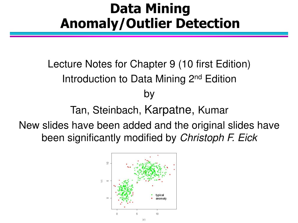
Uncover insights on anomaly and outlier detection in data mining through lecture notes from Chapter 9 of the book "Introduction to Data Mining 2nd Edition" by Tan, Steinbach, Karpatne, Kumar. These notes have been revised by Christoph F, featuring new slides. Explore the updated content to enhance your knowledge in this specialized area of data analysis.

Download Presentation

Please find below an Image/Link to download the presentation.
The content on the website is provided AS IS for your information and personal use only. It may not be sold, licensed, or shared on other websites without obtaining consent from the author.If you encounter any issues during the download, it is possible that the publisher has removed the file from their server.
You are allowed to download the files provided on this website for personal or commercial use, subject to the condition that they are used lawfully. All files are the property of their respective owners.
The content on the website is provided AS IS for your information and personal use only. It may not be sold, licensed, or shared on other websites without obtaining consent from the author.
E N D
Presentation Transcript
Data Mining Anomaly/Outlier Detection Lecture Notes for Chapter 9 (10 first Edition) Introduction to Data Mining 2nd Edition by Tan, Steinbach, Karpatne, Kumar New slides have been added and the original slides have been significantly modified by Christoph F. Eick
Lecture Organization COSC 3337 Anomaly/Outlier Detection Graphic-based Approaches Model-based One-Class SVM Approach only briefly covered Distance-Based Approaches Reconstuction Error-based approach 1. 2. 3. 4. 5. 10/10/2023 Eick, Tan,Steinbach,Kapatne, Kumar COSC 3337: Data Science I
0. Anomaly/Outlier Detection What are anomalies/outliers? The set of data points that are considerably different than the remainder of the data Variants of Anomaly/Outlier Detection Problems Given a database D, find all the data points x D with anomaly scores greater than some threshold t Given a database D, find all the data points x D having the top-n largest anomaly scores f(x) Given a database D, containing mostly normal (but unlabeled) data points, and a test point x, compute the anomaly score of x with respect to D Applications: Credit card fraud detection, telecommunication fraud detection, network intrusion detection, fault detection, data cleaning, sensor fusion, 10/10/2023 Eick, Tan,Steinbach,Kapatne, Kumar COSC 3337: Data Science I
Anomaly Detection Assumption: There are considerably more normal observations than abnormal observations (outliers/anomalies) in the dataset Challenges How many outliers are there in the data? Method is unsupervised Validation can be quite challenging (just like for clustering) Finding needle in a haystack 10/10/2023 Eick, Tan,Steinbach,Kapatne, Kumar COSC 3337: Data Science I
Anomaly Detection Schemes General Steps Build a profile of the normal behavior Profile can be patterns or summary statistics for the overall population Use the normal profile to detect anomalies Anomalies are observations whose characteristics differ significantly from the normal profile Types of anomaly detection schemes 1. Graphical 2. Model-based, relying on parametric models 3. One-Class SVM Approach 4. Distance-based 5. Profile-based Approaches 10/10/2023 Eick, Tan,Steinbach,Kapatne, Kumar COSC 3337: Data Science I
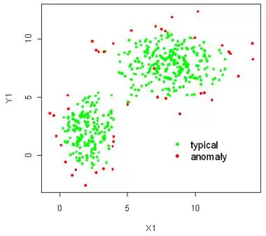
1. Graphical Approaches Idea: user identifies outliers by visual inspection Scatter plot (2-D), Spin plot (3-D) Limitations Time consuming Subjective Data with higher dimensions 10/10/2023 Eick, Tan,Steinbach,Kapatne, Kumar COSC 3337: Data Science I
Box-Plot Approach for Outlier Detection outlier 1.5*IQR IQR Mixture of a graphical and a statistical approach Observations that are more than IQR (e.g. =1.5) above or below the inter-quantile range are outliers. Decent approach for 1D/single attribute outlier detection! Sad news: Cannot be used for multi-variate data! 10/10/2023 Eick, Tan,Steinbach,Kapatne, Kumar COSC 3337: Data Science I
Outlier Detection Example1 10/10/2023 Eick, Tan,Steinbach,Kapatne, Kumar COSC 3337: Data Science I
Anomaly/Outlier Detection (Second Introduction) What are anomalies/outliers? The set of data points that are considerably different than the remainder of the data Natural implication is that anomalies are relatively rare One in a thousand occurs often if you have lots of data Context is important, e.g., freezing temps in July Can be important or a nuisance 10 foot tall 2 year old Unusually high blood pressure 10/10/2023 Eick, Tan,Steinbach,Kapatne, Kumar COSC 3337: Data Science I
Causes of Anomalies Data from different classes Measuring the weights of oranges, but a few grapefruit are mixed in Natural variation Unusually tall people Data errors 200 pound 2 year old 10/10/2023 Eick, Tan,Steinbach,Kapatne, Kumar COSC 3337: Data Science I
Object vs. Attribute Anomalies Many anomalies are defined in terms of a single attribute Height Shape Color Object anomalies are harder to identify as objects are usually described by multiple attributes Can be hard to find an anomaly using all attributes Noisy or irrelevant attributes Object is only anomalous with respect to some attributes However, an object may not be anomalous in any one attribute 10/10/2023 Eick, Tan,Steinbach,Kapatne, Kumar COSC 3337: Data Science I
General Issues: Anomaly Scoring Many anomaly detection techniques provide only a binary categorization An object is an anomaly or it isn t This is especially true of classification-based approaches Other approaches assign a score to each object/pont This score measures the degree to which an object is an anomaly This allows objects to be ranked In general, this is the preferable approach However, in the end, you often need a binary decision Should this credit card transaction be flagged? Still useful to have a score How many anomalies are there? 10/10/2023 Eick, Tan,Steinbach,Kapatne, Kumar COSC 3337: Data Science I
2. Model-Based Anomaly Detection Build a model for the data and see Unsupervised Anomalies are those points that don t fit well Anomalies are those points that distort the model Examples: Statistical distribution Clusters Regression Geometric Graph Supervised Anomalies are regarded as a rare class Need to have training data 10/10/2023 Eick, Tan,Steinbach,Kapatne, Kumar COSC 3337: Data Science I
Additional Anomaly Detection Techniques Proximity-based Anomalies are points far away from other points Can detect this graphically in some cases Density-based Low density points are outliers Pattern matching Create profiles or templates of atypical but important events or objects Algorithms to detect these patterns are usually simple and efficient 10/10/2023 Eick, Tan,Steinbach,Kapatne, Kumar COSC 3337: Data Science I
Model-based Statistical Approaches Fit a parametric model M to the data, capturing the distribution of the data (e.g., normal distribution) Apply a statistical test that depends on Data distribution Parameter of distribution (e.g., mean, variance) Number of expected outliers (confidence limit) Alternatively, rank points by their likelihood with respect to M Data Density Function 10/10/2023 Eick, Tan,Steinbach,Kapatne, Kumar COSC 3337: Data Science I
Normal Distributions One-dimensional Gaussian 8 7 0.1 6 0.09 5 0.08 4 Two-dimensional Gaussian 0.07 3 0.06 2 0.05 1 y 0.04 0 0.03 -1 0.02 -2 -3 0.01 -4 probability density -5 -4 -3 -2 -1 0 1 2 3 4 5 x 16 10/10/2023 Eick, Tan,Steinbach,Kapatne, Kumar COSC 3337: Data Science I
Statistical Approaches: GMM 1. Fit a model M to the dataset D; e.g. A Bivariate Gaussian Model A Bivariate Gaussian Mixture Model Mixture model Wikipedia by running the EM clustering algorithm; see:Expectation maximization algorithm - Wikipedia 2. Plug each point p into the density function dM of model M and compute dM(p) or preferably log(dM(p)), called the log likelihood of p, and add this value as in a new column ols ( outlier score ) to D obtaining D the smaller this value is the more likely p is an outlier with respect M. 3. Sort D in ascending order the first record is the record with the smallest value for log(dM(p)) 4. Remove the top k records from D GMM-Model 10/10/2023 Eick, Tan,Steinbach,Kapatne, Kumar COSC 3337: Data Science I
General Idea EM Algorithm EM Algorithm Gaussian Mixture Models: http://pypr.sourceforge.net/mog.html http://scikit-learn.org/stable/modules/mixture.html Works like K-means 18 10/10/2023 Eick, Tan,Steinbach,Kapatne, Kumar COSC 3337: Data Science I
Parameter of K-Means/GMM Models K-means models are characterized by k centroids EM/Gaussian Mixture Models are characterized by k Gaussian with each Gaussian characterized by: Weight of the particular Gaussian Mean value Covariance Matrix EM-style algorithms: E-Step: Assign objects to clusters (deterministic in the case of K-means; probabilistic in the case of EM) M-Step: updates the model parameters (e.g. centroids in the case of K-means; the mixture parameters in the case of EM) Repeat sequences of E-M steps until there is some convergence Start with an initial assignment of objects to clusters 10/10/2023 Eick, Tan,Steinbach,Kapatne, Kumar COSC 3337: Data Science I
Statistical/Model-based Approaches: 1. Fit a model M to the dataset D; e.g. A Bivariate Gaussian Model A Bivariate Gaussian Mixture Model by running the EM clustering algorithm; see:Expectation maximization algorithm - Wikipedia 2. Plug each point p into the density function dM of model M and compute dM(p) or preferably log(dM(p)), called the log likelihood of p, and add this value as in a new column ols ( outlier score ) to D obtaining D the smaller this value is the more likely p is an outlier with respect M. 3. Sort D in ascending order the first record is the record with the smallest value for log(dM(p)) 4. Perform the remaining tasks using D GMM-Model 10/10/2023 Eick, Tan,Steinbach,Kapatne, Kumar COSC 3337: Data Science I
Density-based: LOF approach Not covered For each point, compute the density of its local neighborhood; e.g. use DBSCAN s approach In anomaly detection, the local outlier factor (LOF) is an algorithm proposed by Markus M. Breunig, Hans-Peter Kriegel, Raymond T. Ng and J rg Sander in 2000 for finding anomalous data points by measuring the local deviation of a given data point with respect to its neighbours.[1] Outliers are points with largest LOF value (measured as point- density/neighbor densities) In the NN approach, p2 is not considered as outlier, while LOF approach find both p1 and p2 as outliers; moreover, some/all points in cluster C1 might be considered as outliers! p2 p1 10/10/2023 Eick, Tan,Steinbach,Kapatne, Kumar COSC 3337: Data Science I
Relative Density Outlier Scores Not covered 6.85 6 C 5 4 1.40 D 3 1.33 2 A 1 Outlier Score 22 10/10/2023 Eick, Tan,Steinbach,Kapatne, Kumar COSC 3337: Data Science I
Limitations of Model-based Approaches Most of the statistical tests are for a single attributes In many cases, data distribution/model may not be known For high dimensional data, it may be difficult to estimate the true density function. However, mixtures of Gaussians and conjunction with EM have been successfully used in practice for some outlier detection tasks that involve multi-variate data. However, very high dimensional data are still a challenge! As alternative to parametric density estimation, non-parametric density-based approaches, such as kernel density estimation have shown some promise; see: https://en.wikipedia.org/wiki/Kernel_density_estimation However, these approaches just provide you with estimated densities but not with a true density function density function; therefore, they are not truly model based, but rather just density- based approaches. 10/10/2023 Eick, Tan,Steinbach,Kapatne, Kumar COSC 3337: Data Science I
Model-based vs Model-free Model-based Approaches Model can be parametric or non-parametric Anomalies are those points that don t fit well Anomalies are those points that distort the model Model-free Approaches Anomalies are identified directly from the data without building a model Often the underlying assumption is that the most of the points in the data are normal Introduction to Data Mining, 2nd Edition Tan, Steinbach, Karpatne, Kumar 4/12/2021 24 10/10/2023 Eick, Tan,Steinbach,Kapatne, Kumar COSC 3337: Data Science I
General Issues: Label vs Score Some anomaly detection techniques provide only a binary categorization Other approaches measure the degree to which an object is an anomaly This allows objects to be ranked Scores can also have associated meaning (e.g., statistical significance) Introduction to Data Mining, 2nd Edition Tan, Steinbach, Karpatne, Kumar 4/12/2021 25 10/10/2023 Eick, Tan,Steinbach,Kapatne, Kumar COSC 3337: Data Science I
3. One-Class SVM Approachfor Outlier Detection Consider a sphere with center a and radius R Minimize R and the error resulting from points outside the sphere their error is their distance to the sphere. Lowercase greek xiletter, pronounced ksi C + 2 t min R t subject to + 2 t t t x , 0 a R error More information: http://rvlasveld.github.io/blog/2013/07/12/introduction-to-one-class-support-vector-machines/ 10/10/2023 Eick, Tan,Steinbach,Kapatne, Kumar COSC 3337: Data Science I
One Class SVM with Kernel Functions Again kernel functions/mapping to a higher dimensional space can be employed in which case the class boundary shapes change as depicted. 10/10/2023 Eick, Tan,Steinbach,Kapatne, Kumar COSC 3337: Data Science I
4. Distance-based Approaches Approach: Compute the distance between every pair of data points There are various ways to define outliers: Data points for which there are fewer than p neighboring points within a distance r The top n data points whose distance to the kth nearest neighbor is greatest The top n data points whose average distance to the k nearest neighbors is greatest 10/10/2023 Eick, Tan,Steinbach,Kapatne, Kumar COSC 3337: Data Science I
One Nearest Neighbor - One Outlier D 2 1.8 1.6 1.4 1.2 1 0.8 0.6 0.4 10/10/2023 Eick, Tan,Steinbach,Kapatne, Kumar COSC 3337: Data Science I
One Nearest Neighbor - Two Outliers 0.55 D 0.5 0.45 0.4 0.35 0.3 0.25 0.2 0.15 0.1 0.05 10/10/2023 Eick, Tan,Steinbach,Kapatne, Kumar COSC 3337: Data Science I
Five Nearest Neighbors - Small Cluster 2 D 1.8 1.6 1.4 1.2 1 0.8 0.6 0.4 10/10/2023 Eick, Tan,Steinbach,Kapatne, Kumar COSC 3337: Data Science I
Five Nearest Neighbors - Differing Density D 1.8 1.6 1.4 1.2 1 0.8 0.6 0.4 0.2 10/10/2023 Eick, Tan,Steinbach,Kapatne, Kumar COSC 3337: Data Science I
Reconstruction-Error Based Approaches Based on assumptions there are patterns in the distribution of the normal class that can be captured using lower-dimensional representations Reduce data to lower dimensional data E.g. Use Principal Components Analysis (PCA) or Auto-encoders Measure the reconstruction error for each object The difference between original and reduced dimensionality version Covered in more detail in November 2023! Introduction to Data Mining, 2nd Edition Tan, Steinbach, Karpatne, Kumar 4/12/2021 33 10/10/2023 Eick, Tan,Steinbach,Kapatne, Kumar COSC 3337: Data Science I
Reconstruction Error Let ? be the original data object Find the representation of the object in a lower dimensional space Project the object back to the original space Call this object ? Reconstruction Error(x x)= x x x x Objects with large reconstruction errors are anomalies Introduction to Data Mining, 2nd Edition Tan, Steinbach, Karpatne, Kumar 4/12/2021 34 10/10/2023 Eick, Tan,Steinbach,Kapatne, Kumar COSC 3337: Data Science I
Basic Architecture of an Autoencoder An autoencoder is a multi-layer neural network The number of input and output neurons is equal to the number of original attributes. Introduction to Data Mining, 2nd Edition Tan, Steinbach, Karpatne, Kumar 4/12/2021 35 10/10/2023 Eick, Tan,Steinbach,Kapatne, Kumar COSC 3337: Data Science I
Strengths and Weaknesses Does not require assumptions about distribution of normal class Can use many dimensionality reduction approaches The reconstruction error is computed in the original space This can be a problem if dimensionality is high Introduction to Data Mining, 2nd Edition Tan, Steinbach, Karpatne, Kumar 4/12/2021 36 10/10/2023 Eick, Tan,Steinbach,Kapatne, Kumar COSC 3337: Data Science I


")