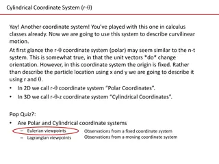
Curvilinear Motion in 3D Space


Curvilinear Motion

To visualize things in 3-dimensional space you are probably most familiar
with the x-y-z coordinate system (cartesian). We covered rectilinear motion
the last few lectures, and now we will move to 3D space
We can describe a position vector (
r
) that has the tail at the origin, and the
head at the particle position.


The coordinate system does *not* change the following relationships
between position, velocity, and acceleration. As we explore different
coordinate systems, the equations may change, but the foundational
relationships do not.


General Curvilinear Motion

Curvilinear Motion:

12.4


Curved motion in 3 dimensions (3D)

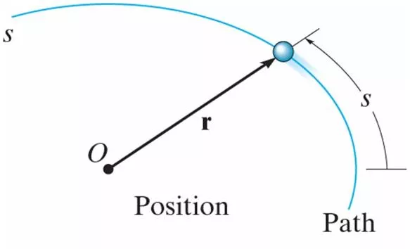
Position:

Position of a
particle
measured from
fixed point 0 described with a vector:

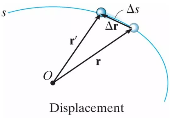
Displacement:

Change in position.

position vector is a
function of time


General Curvilinear Motion
12.4
Velocity:
Change in vector position.
average velocity:
instantaneous velocity:
instantaneous velocity is
the derivative of position
common units: in/s, ft/s, m/s
velocity is always
tangent to the curve
velocity magnitude (speed):
General Curvilinear Motion
12.4
Acceleration:
Change in vector velocity.
average acceleration:
instantaneous acceleration:
instantaneous acceleration
is the derivative of velocity
common units: in/s
2
, ft/s
2
, m/s
2
A
hodograph
is a plot of velocity vectors
with their tails located at a fixed point
0’
Acceleration points to the “inside”
or “concave side” of the path
Curvilinear Motion: Rectangular Components
Position:
12.5
A particle located at
(x,y,z
) from origin
0
.
position:
magnitude:
direction:
(unit vector)
Curvilinear Motion: Rectangular Components
12.5
Velocity:
Velocity has direction and magnitude. Velocity is always tangent
to the path. Tail emanates from the particle.
vector
velocity:
magnitude:
direction:
(unit vector)
Curvilinear Motion: Rectangular Components
12.5
Acceleration:
Acceleration has direction and magnitude. Acceleration points
towards the inside of the path curve.
vector
acceleration:
magnitude:
direction:
(unit vector)
Motion of a Projectile
12.6
Horizontal
Motion:
Free-flight motion of a projectile using rectangular components.
Constant Acceleration
Equations:
Vertical
Motion:
constant acceleration (no variation with altitude or elevation)
Assumptions for Analysis:
no friction/damping from air (no forces act on particle during flight)
For projectile flight, use:
In-Class Practice Problem 1
What do you notice about this problem?
Key words?
What information do you know?
What are you trying to find?
How to you approach the problem?
What equation(s) will you use?
In-Class Practice Problem 1
In-Class Practice Problem 2
What do you notice about this problem?
Key words?
What information do you know?
Does the lack of numbers bother you?
What are you trying to find?
How to you approach the problem?
What equation(s) will you use?
In-Class Practice Problem 2
In-Class Practice Problem 3
What do you notice about this problem?
Key words or information?
What information do you know?
What are you trying to find?
How to you approach the problem?
What equation(s) will you use?
In-Class Practice Problem 3
Horizontal
Motion:
In-Class Practice Problem 3
Vertical
Motion:
In-Class Practice Problem 3
curvilinear motion in 3D space involves describing particle position using a position vector, exploring relationships between position, velocity, and acceleration, and visualizing motion through coordinate systems. This concept delves into position vectors, displacement, velocity - both average and instantaneous, acceleration, and rectangular components of motion. The discussion covers how velocity and acceleration are always tangent to the path, hodographs, and direction and magnitude of velocity. Overall, it provides a comprehensive overview of motion in three-dimensional space.

Download Presentation

Please find below an Image/Link to download the presentation.
The content on the website is provided AS IS for your information and personal use only. It may not be sold, licensed, or shared on other websites without obtaining consent from the author.If you encounter any issues during the download, it is possible that the publisher has removed the file from their server.
You are allowed to download the files provided on this website for personal or commercial use, subject to the condition that they are used lawfully. All files are the property of their respective owners.
The content on the website is provided AS IS for your information and personal use only. It may not be sold, licensed, or shared on other websites without obtaining consent from the author.
E N D
Presentation Transcript
Curvilinear Motion To visualize things in 3-dimensional space you are probably most familiar with the x-y-z coordinate system (cartesian). We covered rectilinear motion the last few lectures, and now we will move to 3D space We can describe a position vector (r) that has the tail at the origin, and the head at the particle position. The coordinate system does *not* change the following relationships between position, velocity, and acceleration. As we explore different coordinate systems, the equations may change, but the foundational relationships do not.
12.4 General Curvilinear Motion Curvilinear Motion: Curved motion in 3 dimensions (3D) Position of a particle measured from fixed point 0 described with a vector: Position: ( ) t position vector is a function of time = r r Displacement: Change in position. = + r = r r r r r ' or '
12.4 General Curvilinear Motion Velocity: Change in vector position. r = v average velocity: common units: in/s, ft/s, m/s avg t r = v lim t d dt instantaneous velocity: t 0 r instantaneous velocity is the derivative of position ( ) = v EQ 12- 7 velocity is always tangent to the curve dr will be tangent to the curve, so will be tangent to the curve v velocity magnitude (speed): ds dt = = v v
12.4 General Curvilinear Motion Acceleration: Change in vector velocity. v = a common units: in/s2, ft/s2, m/s2 average acceleration: avg t v A hodograph is a plot of velocity vectors with their tails located at a fixed point 0 = a lim t d dt instantaneous acceleration: t 0 v dv will be tangent to the hodograph, so will be tangent to the hodograph a instantaneous acceleration is the derivative of velocity ( ) = a EQ 12- 9 Acceleration points to the inside or concave side of the path
12.5 Curvilinear Motion: Rectangular Components A particle located at (x,y,z) from origin 0. Position: ( ) = + + r i j k EQ 12- 10 x y z position: = + + r x y z 2 2 2 magnitude: = direction: (unit vector) u r r r
12.5 Curvilinear Motion: Rectangular Components Velocity has direction and magnitude. Velocity is always tangent to the path. Tail emanates from the particle. Velocity: r d dt d dt d dt d dt d dt dx dt dy dt dz dt = = = vector velocity: ( ) x ( ) y ( ) = = + + = + + v i j k i j k i j k , , ( ) z f t r v v v x y z ( ) = = + + v i j k x EQ 12-11 v v v ( ) x y z EQ 12-12 y z = + + v v v y 2 x 2 y 2 z magnitude: direction: (unit vector) = u v v v
12.5 Curvilinear Motion: Rectangular Components Acceleration has direction and magnitude. Acceleration points towards the inside of the path curve. Acceleration: v d dt vector acceleration: ( ) = = = a a a x y z = = + + a i j k EQ 12-13 a a a x x y z ( ) EQ 12-14 y z = + + a a a a 2 x 2 y 2 z magnitude: direction: (unit vector) = u a a a
12.6 Motion of a Projectile Free-flight motion of a projectile using rectangular components. Assumptions for Analysis: constant acceleration (no variation with altitude or elevation) no friction/damping from air (no forces act on particle during flight) = + + + v v x x = = a t v t ??= ? = 9.81 m s2= 32.2 ft Constant Acceleration Equations: 0 c + 1 2 x x a t 2 s2 0 2 0 0 a c ( ) 2 v v 2 0 c For projectile flight, use: = = 0 & a a g x y ( ) v = v Horizontal Motion: 0 x x x = x ( ) v + t 0 0 x = = = ( ) v y v v gt 0 y y y Vertical Motion: + 1 2 ( ) v t gt 2 0 0 y ( ) 2 ( g y y ) v 2 y 2 y 0 0
In-Class Practice Problem 1 What do you notice about this problem? Key words? What information do you know? What are you trying to find? How to you approach the problem? What equation(s) will you use?
In-Class Practice Problem 2 What do you notice about this problem? Key words? What information do you know? Does the lack of numbers bother you? What are you trying to find? How to you approach the problem? What equation(s) will you use?
In-Class Practice Problem 2 = + + = + + v v v y a a a a 2 x 2 y 2 z 2 x 2 y 2 z
In-Class Practice Problem 3 What do you notice about this problem? Key words or information? What information do you know? What are you trying to find? How to you approach the problem? What equation(s) will you use?
In-Class Practice Problem 3 ( ) v = v Horizontal Motion: 0 x x x = x ( ) v + t 0 0 x
In-Class Practice Problem 3 ??= (?0)? ?? ? = ?0+ (?0)?? 1 Vertical Motion: 2??2