Correlation and Covariance in Business Analytics
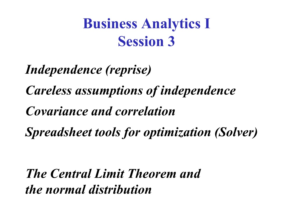
Independence (reprise)
Careless assumptions of independence
Covariance and correlation
Spreadsheet tools for optimization (Solver)
The Central Limit Theorem and
the normal distribution
Business Analytics I
Session 3
Predicting the Results of the
2012 U.S. Presidential Election
See InTrade-2012.xls.
Meadow’s Law: Are crib deaths
independent events?
Beware Unwarranted Assumptions of Independence
Sir Samuel Roy Meadow
(born 1933) is a British pediatrician and professor, who rose to initial
fame for his 1977 academic paper on the now controversial Munchausen Syndrome by Proxy
(MSbP). He was knighted for this work. He endorsed the dictum that
“one sudden infant death
is a tragedy, two is suspicious and three is murder, until proved otherwise“
in his book
ABC of
Child Abuse
[1]
and this became known as Meadow's Law and at one time was widely adopted by
social workers and child protection agencies (such as the NSPCC) in Britain.
He appeared as an expert witness for the prosecution in several trials, in at least one of which his
testimony played a crucial part in a wrongful conviction for murder. The British General
Medical Council (GMC) struck off Meadow from the British Medical Register after he was
found to have offered “erroneous” and “misleading” evidence in the Sally Clark case. Clark was
a lawyer wrongly convicted in 1999 of the murder of her two baby sons, largely on the basis of
Meadow's evidence; her conviction was quashed in 2003 after she had spent three years in jail.
By the time he gave evidence at Sally Clark's trial, Roy Meadow claimed to have found 81 cot
deaths which were in fact murder, but he had destroyed the data.
Amongst the prosecution
team was Meadow, whose evidence included a soundbite which was to provoke much
argument: he testified that the odds against two cot deaths occurring in the same family
was 73,000,000:1, a figure which he obtained by squaring the observed ratio of live-births
to cot deaths in affluent non-smoking families (approximately 8,500:1).
The jury returned a
10/2 majority verdict of "guilty".
“Bad Debt” patterns
Did you notice any patterns in the Bad Debt data?
The 200 transactions that became bad debts averaged $7,443 per invoice.
The 9800 that were eventually paid averaged only $4,332 per invoice.
What was the effect of separating the data for small/large transactions?
The 4,533 “small” (sub-$4000) invoices that were eventually paid were
paid off, on average, in about 94 days. The “large” invoices took, on
average, about 10 days longer.
More strikingly, the 9,679 paid-off invoices below $9000 were paid, on
average, in a bit less than 97 days … and the 121 above $9000 averaged
more than 298 days to payment.
Generally, how might we measure the probabilistic linkage between
random variables? For example, how might we assess whether they tend
to be “large” together, and “small” together?
Dependence and Covariance
If two random variables are
not
independent, do they tend to be large together (and
small together)? Or when one is large, is the other typically small (and vice versa)?
Definition: The
covariance
of random variables X and Y is
Cov(X,Y) = E[ (X
–
E[X]) · (Y
–
E[Y]) ]
= E[XY]
– E[X]·E[Y] .
(The two expressions are algebraically the same.)
A positive covariance corresponds to “typically big together, and small together.”
A negative covariance corresponds to “typically, when one is big, the other is small.”
Independent random variables have a covariance of 0.
Emphatically: A covariance of 0 does
NOT
imply independence.
Correlation
It is easier to interpret covariance after a rescaling:
The
correlation
of two random variables is
Corr(X,Y) = Cov(X,Y) / (StDev(X)·StDev(Y)) .
Just as we use both variance (for calculations) and standard deviation (for
interpretation), we use covariance (for calculations) and correlation (for
interpretation).
Specifically, the correlation between two random variables is a
dimensionless measure of the
strength
of the
linear
relationship between
those
two
variables. It takes values between -1 and 1.
Correlation
... beware
Definition
The
correlation
between two random variables
is a dimensionless number between 1 and -1.
Interpretation
Correlation measures the
strength
of the
linear
relationship between
two
variables.
•
Strength
–
not the slope
•
Linear
–
misses nonlinearities completely
•
Two
–
shows only “shadows” of multidimensional
relationships
A correlation of +1 would
arise only if all of the
points lined up perfectly.
Stretching the diagram horizontally or
vertically would change the perceived
slope, but not the correlation.
Correlation measures the
“tightness” of the clustering
about a single line.
A positive correlation
signals that large values of
one variable are typically
associated with large
values of the other.
A negative correlation
signals that large values of
one variable are typically
associated with small
values of the other.
Independent random
variables have a
correlation of 0.
But a correlation of 0
most certainly does
not
imply
independence.
Indeed, correlations can
completely miss
nonlinear relationships.
Back to Bad Debt
Consider the data provided in
the Bad Debt homework exercise.
Restrict attention to the invoices that were paid (98% of data).
Let I = Invoice amount and
D
= days to pay.
Among paid invoices, is the tendency for
I
and
D
to vary in the
same
or
opposite
direction?
We can calculate E(I) and E(D) (using Excel’s =AVERAGE(range) function
twice) and E(ID) (using =SUMPRODUCT(range)/COUNT(range) ).
Cov(I,D) = E(ID) – E(I)·E(D) = 25636 (dollar-days)
Is this a
strong
relationship? (Excel’s =STDEV(range) function is useful here.)
Corr
(I,D) = Cov(I,D) / (2463.9·93.6) =
0.111
Corr(Google searches for “Vodka”,
Google searches for “SD cards”) = 0.9400
The
correlation
comes from
common
calendar
peaks: a
small one in
June and a
large one in
December.
Consider
advertising
and sales
(for a
seasonal
product)!
Correlation doesn’t imply Causality!
The Variance of a Sum
Tattoo this somewhere on your body:
Var(X+Y) =
Var(X
) + Var(Y) + 2·Cov(X,Y)
.
More generally,
Var(X+Y+Z) = Var(X)+Var(Y)+Var(Z) + 2·Cov(X,Y)+2·Cov(X,Z)+2·Cov(Y,Z) .
and most generally, the variance of a sum is the sum of the individual variances, plus
twice all of the pairwise covariances.
Portfolio Balancing
See portfolios.xls
Next
You are about to learn one of the handful of fundamental facts that
make the universe what it is.
It’s right up there with the inverse square law of gravity, Maxwell’s
equations, the Theory of Relativity, the Law of Large Numbers, and
the existence of the Higgs boson.
It is used in every branch of science, and every functional area of
management.
“I know of scarcely anything so apt to impress the imagination as the
wonderful form of cosmic order expressed by [what you are about to
learn]. [It] would have been personified by the Greeks if they had known
of it. It reigns with serenity and complete self-effacement amidst the
wildest confusion. The larger the mob, the greater the apparent anarchy,
the more perfect is its sway. It is the supreme law of unreason.”
- Sir Francis Galton
What do these problems have in common?
A firm needs to set aside funds to satisfy potential warranty claims for one
product. The firm wants to minimize these funds, but also have a reasonable
chance that the funds will be sufficient to cover all claims.
A firm wants to keep its inventory levels down, but also limit the odds it
runs out of stock in the next month.
Quality control: A pharmaceutical company finds a pallet of drug vials to be
0.31kg underweight. How likely is this under normal conditions? Or when
their vial injector is partly clogged? (
You will see this example in OM-430
)
A casino offers a loss-triggered rebate to a high stakes player. They want to
find the probability that they will have to pay the rebate to that customer.
What the problems had in common
Each problem had these elements…
Large number
of
independent
individual trials
;
Customer purchases, warranty claims, vial weights,
or
gambles.
Repetition
: Comparable
uncertainty
about each of the
individual trials;
Customers indistinguishable from each other, drug vials
coming from same machine, etc.
Summing
: We only really care about the aggregate
total
outcome of these individual trials.
Total of demand, warranty claims, pallet weight, total
winnings.
The Central Limit Theorem
Whenever you sum a bunch of independent random
variables (with comparable variances), no matter what
their individual distributions may be, the result will be
approximately
normally distributed.
How big is “a bunch”?
Empirical studies have shown
that interpreting “a bunch” as
a couple of dozen or more
works quite well.
We illustrate the probability
distribution of a normally-
distributed random variable
through a diagram, where the
total area beneath the curve is 1,
and the probability of the
normal variate lying in any
range is the area above that
range.
The normal distribution
What you needn’t concern yourself with:
The height of the curve at any point
x
(a.k.a. the
density function
) is:
What you do need to know:
Normal distributions are
completely described
by their
expected value
and
standard
deviation
.
Normal distribution “rules of thumb”
P(within one standard deviation of EV) = 2/3.
P(within two standard deviations of EV) = 95%.
P(within three standard deviations of EV) = 99.7%.
P(within four standard deviations of EV) = 99.994%.
The normal distribution in Excel
Excel commands
=NORMDIST(
X
, expected value, standard deviation, TRUE)
gives the probability that you get a value no higher than
X
=NORMINV(probability, expected value, standard deviation)
gives the value
X
corresponding to the stated probability
See also: NORMSDIST, NORMSINV (when EV=0, SD=1)
Newer Excel versions: NORM.DIST, NORM.INV, etc., are identical to these commands.
X
Explore the concepts of covariance and correlation in business analytics to understand the relationship between random variables. Delve into how these measures help analyze dependence between variables, differentiate between independence and covariance, and interpret correlation as a dimensionless measure of linear relationships. Gain insights into predicting outcomes and identifying patterns using statistical tools in spreadsheet optimization.

Download Presentation

Please find below an Image/Link to download the presentation.
The content on the website is provided AS IS for your information and personal use only. It may not be sold, licensed, or shared on other websites without obtaining consent from the author.If you encounter any issues during the download, it is possible that the publisher has removed the file from their server.
You are allowed to download the files provided on this website for personal or commercial use, subject to the condition that they are used lawfully. All files are the property of their respective owners.
The content on the website is provided AS IS for your information and personal use only. It may not be sold, licensed, or shared on other websites without obtaining consent from the author.
E N D
Presentation Transcript
Business Analytics I Session 3 Independence (reprise) Careless assumptions of independence Covariance and correlation Spreadsheet tools for optimization (Solver) The Central Limit Theorem and the normal distribution
Predicting the Results of the 2012 U.S. Presidential Election See InTrade-2012.xls.
Bad Debt patterns Did you notice any patterns in the Bad Debt data? The 200 transactions that became bad debts averaged $7,443 per invoice. The 9800 that were eventually paid averaged only $4,332 per invoice. What was the effect of separating the data for small/large transactions? The 4,533 small (sub-$4000) invoices that were eventually paid were paid off, on average, in about 94 days. The large invoices took, on average, about 10 days longer. More strikingly, the 9,679 paid-off invoices below $9000 were paid, on average, in a bit less than 97 days and the 121 above $9000 averaged more than 298 days to payment. Generally, how might we measure the probabilistic linkage between random variables? For example, how might we assess whether they tend to be large together, and small together?
Dependence and Covariance If two random variables are not independent, do they tend to be large together (and small together)? Or when one is large, is the other typically small (and vice versa)? Definition: The covariance of random variables X and Y is Cov(X,Y) = E[ (X E[X]) (Y E[Y]) ] = E[XY] E[X] E[Y] . (The two expressions are algebraically the same.) A positive covariance corresponds to typically big together, and small together. A negative covariance corresponds to typically, when one is big, the other is small. Independent random variables have a covariance of 0. Emphatically: A covariance of 0 does NOT imply independence.
Correlation It is easier to interpret covariance after a rescaling: The correlation of two random variables is Corr(X,Y) = Cov(X,Y) / (StDev(X) StDev(Y)) . Just as we use both variance (for calculations) and standard deviation (for interpretation), we use covariance (for calculations) and correlation (for interpretation). Specifically, the correlation between two random variables is a dimensionless measure of the strength of the linear relationship between those two variables. It takes values between -1 and 1.
Correlation ... beware
Definition Cov ) Y , X ( = Corr ) Y , X ( StdDev ) X ( StdDev ) Y ( The correlation between two random variables is a dimensionless number between 1 and -1.
Interpretation Correlation measures the strength of the linear relationship between two variables. Strength not the slope Linear misses nonlinearities completely Two shows only shadows of multidimensional relationships
A correlation of +1 would arise only if all of the points lined up perfectly. Stretching the diagram horizontally or vertically would change the perceived slope, but not the correlation.
A positive correlation signals that large values of one variable are typically associated with large values of the other. Correlation measures the tightness of the clustering about a single line.
A negative correlation signals that large values of one variable are typically associated with small values of the other.
Independent random variables have a correlation of 0.
But a correlation of 0 most certainly does not imply independence. Indeed, correlations can completely miss nonlinear relationships.
Back to Bad Debt Consider the data provided in the Bad Debt homework exercise. Restrict attention to the invoices that were paid (98% of data). Let I = Invoice amount and D = days to pay. Among paid invoices, is the tendency for I and D to vary in the same or opposite direction? We can calculate E(I) and E(D) (using Excel s =AVERAGE(range) function twice) and E(ID) (using =SUMPRODUCT(range)/COUNT(range) ). Cov(I,D) = E(ID) E(I) E(D) = 25636 (dollar-days) Is this a strongrelationship? (Excel s =STDEV(range) function is useful here.) Corr(I,D) = Cov(I,D) / (2463.9 93.6) = 0.111
Corr(Google searches for Vodka, Google searches for SD cards ) = 0.9400 The correlation comes from common calendar peaks: a small one in June and a large one in December. Consider advertising and sales (for a seasonal product)!
The Variance of a Sum Tattoo this somewhere on your body: Var(X+Y) = Var(X) + Var(Y) + 2 Cov(X,Y) . More generally, Var(X+Y+Z) = Var(X)+Var(Y)+Var(Z) + 2 Cov(X,Y)+2 Cov(X,Z)+2 Cov(Y,Z) . and most generally, the variance of a sum is the sum of the individual variances, plus twice all of the pairwise covariances.
Portfolio Balancing See portfolios.xls
Next You are about to learn one of the handful of fundamental facts that make the universe what it is. It s right up there with the inverse square law of gravity, Maxwell s equations, the Theory of Relativity, the Law of Large Numbers, and the existence of the Higgs boson. It is used in every branch of science, and every functional area of management. I know of scarcely anything so apt to impress the imagination as the wonderful form of cosmic order expressed by [what you are about to learn]. [It] would have been personified by the Greeks if they had known of it. It reigns with serenity and complete self-effacement amidst the wildest confusion. The larger the mob, the greater the apparent anarchy, the more perfect is its sway. It is the supreme law of unreason. - Sir Francis Galton
What do these problems have in common? A firm needs to set aside funds to satisfy potential warranty claims for one product. The firm wants to minimize these funds, but also have a reasonable chance that the funds will be sufficient to cover all claims. A firm wants to keep its inventory levels down, but also limit the odds it runs out of stock in the next month. Quality control: A pharmaceutical company finds a pallet of drug vials to be 0.31kg underweight. How likely is this under normal conditions? Or when their vial injector is partly clogged? (You will see this example in OM-430) A casino offers a loss-triggered rebate to a high stakes player. They want to find the probability that they will have to pay the rebate to that customer.
What the problems had in common Each problem had these elements Large number of independent individual trials; Customer purchases, warranty claims, vial weights,or gambles. Repetition: Comparable uncertainty about each of the individual trials; Customers indistinguishable from each other, drug vials coming from same machine, etc. Summing: We only really care about the aggregate total outcome of these individual trials. Total of demand, warranty claims, pallet weight, total winnings.
The Central Limit Theorem Whenever you sum a bunch of independent random variables (with comparable variances), no matter what their individual distributions may be, the result will be approximatelynormally distributed. We illustrate the probability distribution of a normally- distributed random variable through a diagram, where the total area beneath the curve is 1, and the probability of the normal variate lying in any range is the area above that range. How big is a bunch ? Empirical studies have shown that interpreting a bunch as a couple of dozen or more works quite well.
The normal distribution What you needn t concern yourself with: The height of the curve at any point x (a.k.a. the density function) is: What you do need to know: Normal distributions are completely described by their expected value and standarddeviation.
Normal distribution rules of thumb P(within one standard deviation of EV) = 2/3. P(within two standard deviations of EV) = 95%. P(within three standard deviations of EV) = 99.7%. P(within four standard deviations of EV) = 99.994%.
The normal distribution in Excel X Excel commands =NORMDIST(X, expected value, standard deviation, TRUE) gives the probability that you get a value no higher than X =NORMINV(probability, expected value, standard deviation) gives the value X corresponding to the stated probability See also: NORMSDIST, NORMSINV (when EV=0, SD=1) Newer Excel versions: NORM.DIST, NORM.INV, etc., are identical to these commands.