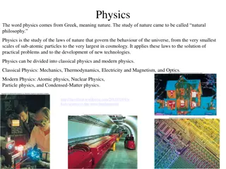
Conservation Principles in Fluid Dynamics and Classical Mechanics
Conservation principles play a significant role in fluid dynamics and classical mechanics. In fluid dynamics, conservation of mass, momentum, and energy are crucial for understanding fluid behavior. Classical mechanics, on the other hand, relies on Newton's laws to describe motion and energy conservation. This comprehensive overview delves into the equations, examples, and applications illustrating the conservation of mass, momentum, and energy in both fluid dynamics and classical mechanics.

Download Presentation

Please find below an Image/Link to download the presentation.
The content on the website is provided AS IS for your information and personal use only. It may not be sold, licensed, or shared on other websites without obtaining consent from the author.If you encounter any issues during the download, it is possible that the publisher has removed the file from their server.
You are allowed to download the files provided on this website for personal or commercial use, subject to the condition that they are used lawfully. All files are the property of their respective owners.
The content on the website is provided AS IS for your information and personal use only. It may not be sold, licensed, or shared on other websites without obtaining consent from the author.
E N D
Presentation Transcript
Conservation of mass, momentum and energy in fluid dynamics
Classical mechanics (Newtonian) The motion of a point mass is governed by Newton s second law 2 r d = F mdt 2 This is a set of ordinary differential equations (ODEs): 1 m = ( , , , , , , ) F t x y z x y z x x 1 m = ( , , , , , , ) F t x y z x y z y y 1 m = ( , , , , , , ) F t x y z x y z z z
Classical mechanics (Newtonian) The equations of motion are supplemented with the initial conditions (for the position and velocity of the point mass at the initial time t = t0) = = r r ( ) t , ( ) t , 0 0 0 0 that is = = = = ( ) ( ) x t , ( ) y t , ( ) , , x t x v y = z t z 0 0 0 ( ) y t 0 0 z t 0 = , ( ) . v v 0 0 0 0 0 0 x y z
Classical mechanics (Newtonian) Example: One-body problem: determine the motion of a point mass (m) moving in the gravity force field produces by a stationary mass (M). Let the mass M is placed in the center of a coordinate system XYZ. Then the equation of motion for the point mass m is 2 r d dt mM r = 2 r m G 2 This is a set of the following equations in 3D: 2 d x dt d y dt d z dt x = , GM In fact, this system can be reduced to 2D (planar) problem, because the (x(t),y(t),z(t)) lies in the plane defined by the initial position and velocity. + + 2 2 2 2 3/2 ) ( x y z trajectory 2 y = , GM + + 2 2 2 2 3/2 ) ( x y z 2 x = . GM + + 2 2 2 2 3/2 ) ( x y z
Classical mechanics (Newtonian) Example (cond.) 2 d x dt d y dt d z dt x = , GM + + 2 2 2 2 3/2 ) ( x y z 2 y = , GM + + 2 2 2 2 3/2 ) ( x y z 2 x = . GM + + 2 2 2 2 3/2 ) ( x y z Possible orbits, due to universal gravity, of a small mass around a single large mass.
Classical mechanics (Newtonian) Energy in classical mechanics appears as follows: when the force is conservative (rot F = 0), then it can be expressed as the gradient of a scalar function V = F . V This function is called the potential of the force or simply the potential energy. It is also denoted by Ep. Then the mechanical energy E is defined as the sum of the kinetic and potential energy = + = 1 2 + 2 . E E E m V kin pot Important property of E is that this quantity is preserved: for any motion r(t) in the force field F it holds that ( ( )) E t const = r . We say that the mechanical energy is conserved.
Classical mechanics (Newtonian) Example: Motion of a point mass near the Earth surface = = , E V mgh p hence 1 2 = + = + = 2 E E E m mgh const kin pot The notion of such conserved quantity helps solving many problems. For example, what is the maximum height that a stone thrown vertically upward will attain if the initial velocity is v0? 1 2 1 2 = + = = + = + 2 2 0 0 E E E const m mg m mg h 0 max kin pot 2 1 2 = = 2 0 g . m mg h max h 0 max 2
Classical mechanics (Newtonian) Example: In the motion of a point mass (m) in the gravitational field of a big stationary planet/star (M) the potential energy of the mass m is Mm r = , E G p hence 1 2 mM r = + = = 2 E E E m G const kin pot 2 In this particular case the mass m disappears as we can divide by it to obtain 2 M r = G const 2 2 Even if we do not know the solution r(t) we know that the above quantity must be constant with respect to time durrng the motion.
Classical mechanics (Newtonian) If a constant force is applied to a particle and a displacement is r , the work is defined as W = F r In general case when the force may vary in space the work is defined by the line integral W = F r d AB where ABis a path along which the mass is moved from point A to B. Note that in general this definition implies that the work may depend on the path. This is not true if the force is conservative. In the case of conservative force we have F = = ( ) B r ( ) A r r W d E E AB
Fluid mechanics (concept of a continuum) Materials (solids, liquids and gases) are composed of molecules separated by empty space. But the continuum model as a mathematical concept assumes that material exists as a continuous entity. It means that the matter in the body is continuously distributed and fills the entire region of space it occupies. A continuum body can, for example, be infinitely sub-divided into smaller and smaller elements preserving properties of the bulk material. It also means that two points in such body may be close at arbitrary small distance. Due to these assumption we can consider physical quantities (density, pressure, velocity, forces etc.) as defined at every point as continuous functions of space position and that space derivatives can be also defined. Example (density). A function (x,y,z,t) is defined at every point (x,y,z) and is continuous. The meaning of this function is as follows: (x,y,z) W = ( , , , ) x y z t dxdydz = ( , ) r ( , ) m W t t dV W W is the mass contained in the region W.
Fluid mechanics Let be a region in two dimensional (2D) or three dimensional (3D) space filled with a fluid (gas or liquid). Our object is to describe the motion of such a fluid. Let r be a point and consider the particle of fluid moving through r at time t. In a standard Euclidean coordinates system in space, we write r = (x, y, z). This particle traverses a well-defined trajectory r(t)=(x(t),y(t),z(t). Let v(r, t) denote the velocity of the particle of fluid that is moving through r at time t. Thus, for each fixed time, v is a vector field on , as in figure below. We call v the (spatial) velocity field of the fluid.
Fluid mechanics (mass conservation) We will use the notion of some region W which will move according to the velocity field. The symbol Wtmeans the set of points of the initial set (region) W displaced to new location after time t. Thus we have W0= W. The obvious property of such defined set Wtis = ( ) ( ) m W m W 0 t This formula is just a statement of the mass conservation law. It is also called the continuity equation or mass balance equation. Let us notice that it can also be written as = dV const W t d dt = 0 dV W t
Fluid mechanics (mass conservation) The form of mass conservation law from the previous slide d dt = = or 0 dV const dV W W t t may be converted to more useful differential form. It can be done in two ways: (1) from the above integral form by applying Reynold s transport theorem; (2) By direct application of Gauss divergence theorem. Th final form is + = v div( ) 0 t Some textbooks use the notation for the divergence operator: u = div u.
Fluid mechanics (material derivative) The material derivative of a scalar function f(t,r) in the region filled with a moving fluid with the velocity field v(t,r) is defined as Df Dt f t = + ( : ) f It takes into account the fact that the fluid is moving and that the positions of fluid particles change with time. Thus, if r(t) = [x(t), y(t), z(t)] describes the movement of a fluid particle (the path followed by the fluid particle), then the change of any quantity f along this path can be computed as follows dx 3 d dt f t f x dt = + = ( , ( )) t r i ( , ( ), ( ), ( )) f t x t y t z t t = 1 f z i i ( ) dt ( ) dt ( ) dt f x dx t f y dy t dz t Df Dt + + = + = ( , ( )) t r ( , ( )) t r ( , ( )) t r ( ) t t t f t ( , ( )) t r ( , ( )) t r t t Hence we can write for the change of function f(t,r) along the path r(t): d dt Df Dt = ( , ( )) f t r ( , ( )). t r t t
Fluid mechanics (ideal fluid) For any continuum, forces acting on a piece of material are of two types: External, or body, forces such as gravity, intertial (pseudoforce) , a magnetic field, which exert a force per unit volume on the continuum forces of stress, whereby the piece of material is acted on by forces across its surface by the rest of the continuum. An ideal fluid has the following property: For any motion of the fluid there is a scalar function p(t,r) called the pressure such that if S is a surface in the fluid with a normal vector n, the force of stress exerted across the surface S per unit area at r S at time t is p(t,r)n, i.e. p t r n force across per unit area = ( , ) . S
Fluid mechanics (ideal fluid momentum equation) Intuitively, the absence of tangential forces implies that there is no way for rotation to start in a fluid, nor, if it is there at the beginning, to stop. This may be too much simplification and we can detect physical trouble for ideal fluids because of the abundance of rotation in real fluids (near the oars of a rowboat, in tornadoes, etc.). If W is a region in the fluid at a particular instant of time t, the total force exerted on the fluid inside W by means of stress on its boundary is = r n S ={force on W through the surface S} ( , ) p t . dA W W If e is any fixed vector in space, then the divergence theorem gives = = = = e e S e n e e div( ) ( ) p dA p dV p dV pdV W W W W W hence = S pdV W W
Fluid mechanics (ideal fluid momentum equation) If b(t,r) denotes the given body force per unit mass, then the total body force is = , ={body force on W } b W F b . dV W Thus the total force acting on the fluid domain W in the case of ideal fluid is = + = + + S b b F ( ) ( ) p dV dV p dV , b W W W W W = + F b ( ) p dV W W Hence = + b force per unit volume p
Fluid mechanics (ideal fluid) Now we want to apply Newton s second law for the fluid element W force = mass acceleration Acceleration: let r(t) is the motion of the fluid particle. From the very definition of the velocity we get r d dt = v ( , ( )) t r ( ) t t The acceleration a=d2r/dt2thus 2 r d dt d dt = = a ( , ( )) t r v ( ) t ( ) t t 2 But, by the chain rule one can show v d dt = = + a ( , ( )) t r v v v ( ) t ( ) t t
Fluid mechanics (ideal fluid Eulers equations) Let us summarize: force = mass acceleration force per unit volume = + b p v = = + v a v acceleration t From the above relations we get v + v = + b v p t The above equation is called Euler s equation for ideal fluid. In fact it is the momentum balance for the ideal fluid.
Fluid mechanics (NavierStokes equations) Now we consider a more general fluid than the ideal one. Real fluids possess the phenomenon of viscosity. The microscopic basis of the effect of viscosity is connected with the transfer of momentum between layers of moving fluid. If the forces are only normal to S, there will be no transfer of momentum between the fluid volumes denoted by B1 and B2. However, in reality faster molecules from above (B2) will diffuse across S and impart momentum to the fluid (B1), and, likewise, slower molecules from below S will diffuse across S to slow down the fluid above S. This is how the viscosity arises.
Quantifying the dynamic viscosity In the previous slide the viscosity was explained in the qualitative way. Here is how we can measure it. The dynamic viscosity (sometimes ) of a fluid describes its resistance to shearing flows. In the picture (the speed of the top plate is parallel to the x axis. We see that an external force F is required in order to keep the top plate moving at constant speed v. = = = F A A A y F A = = y
Fluid mechanics (NavierStokes equations) Instead of assuming that (ideal fluid) = ( , ) , t r n force on per unit area S p where n is the normal vector to S, we now assume that (viscous fluid) = + ( , ) r n ( , ) r n force on per unit area S , p t t normal forces possible shear tangential forces ( ) where is the stress tensor which describes the shear forces (tensions) in the fluid. It is called the Cauchy stress tensor. In a fixed coordinate system the tensor stress is just a matrix 3 x 3. Hence the expression n should be understood as the matrix multiplication (n is written here as a column). From this formulation we see that shear force term is linear with respect to n. It is not obvious! It can be proved under a general assumption (continuous dependence on n) and using balance of momentum. This result is called Cauchy s theorem.
Fluid mechanics (NavierStokes equations) As in the case of the ideal fluid we can formulate for viscous fluid Newton s second law for the moving fluid particle Wt d dt = + + n n dV v b ( ) p dA dV W W W t t t internal forces external (body) forces where dV indicates the volume integral and dA is the surface integral. The internal forces acting through surface are now composed of two terms: normal (represented by scalar function p the pressure) and shear/tangential (represented by matrix function the stress tensor). It can be also proved that the stress tensor is symmetric.
Fluid mechanics (NavierStokes equations) To obtain a more specific equation for the motion of the fluid we have to analyze in more detail the stress tensor . The following assumptions are physically sound: depends linearly on the velocity gradients v. is invariant under rotations in space. is symmetric (as was pointed out earlier this can be deduce as a consequence of balance of angular momentum. 1. 2. 3. The velocity gradient is just a matrix of first order space derivatives of all componets of the velocity v=[vx, vy, vz] v v v x x x x y z v v v = v y y y x y z v v v z z z x y z
Fluid mechanics (NavierStokes equations) Under the assumptions 1,2,3 (previous slide) it can be shown that the stress tensor has the following form = (div ) +2 v I D Where and are non-negative parameters characterazing the viscous fluid and v v v v v + + ( ) ( ) 1 2 1 2 y x x x z x y x z x 1 2 ( ) v v v v v + v = + + T v D = ( ) ( ) ( ) 1 2 1 2 y y y x z y x y z y v v v v v + + ( ) ( ) 1 2 1 2 y x z z z z x z y z
Fluid mechanics (NavierStokes equations) If we now employ the transport theorem and the divergence theorem to the balance of momentum with the stress tensor = (div v)I + 2 D after some algebra we will obtain the famous Navier-Stokes equations (NS): v + = + + ) (div ) + v v v v ( ) ( p t This form is for a general fluid at that stage we do not assume incompressibility, so the unknowns are: v(t,r), (t,r), p(t,r). Thus we have five unknown functions, but the NS system gives only three equations. One more equation is obvious it is the mass balance equation + = v div( ) 0 t The fifth equation (for compressible fluid) comes usually in the form of a constitutive relation between pressure, density and temperature: = ( , ). p T
Fluid mechanics (incompressible Navier Stokes equations) Assumption: the viscous fluid is incompressible, i.e. = const. The mass balanace equation gives now 0 + = + div( ) = v v div =0. v div( ) 0 0 0 t and the term ( + ) (div v) vanishes from the NS system. Thus we obtain the Navier Stokes equations for incompressible fluid (usually written with the kinematic viscosity = / >0): v 1 + = + v v v ( ) p t div = 0 v
Fluid mechanics boundary conditions We will consider only two basic boundary conditions. Boundary is denoted by . = v n 0 on 1) The expression means that the normal component of the velocity on the boundary is zero. It is rather obvious statement that the wall is impenetrable. The tangential component may be non-zero (fluid can slip along the wall. This condition is consistent with the inviscid fluid and is used with Euler sequation. = v 0 on 2) This condition says that the velocity on the boundary is completely zero. The tangential component must vanish, hence this is called non-slip boundary condition. It is consistent with viscous fluid ( > 0) and is used in the Navier- Stokes equations.
Fluid mechanics (energy conservation) For any moving fluid region of volume Wtwe can define its energy as 2 = + , E e dV W 2 t W t where is the density, v is the velocity field, and e is the density of internal energy. We identify here = = the kinetic energy of the moving volume Wt 2 E dV kin 2 W t = edV = E the internal energy of the moving volume Wt int W t Now we are interested in how the quantity Wt changes with time when the fluid particle moves in the system. EWt
Fluid mechanics (energy) If we want to move the time derivative under the symbol of integral we must be cautious because the region of integration Wtalso depend on time. It is not stationary! The rate of change with time can be rewritten Reynold s transport theorem 2 2 d dt D Dt + = + e dV e dV 2 2 W W t t where we applied the transport theorem (Reynolds) d dt Df Dt = , f dV dV W W t t valid for any quantity f(t,r)=f(t,x,y,z) that may depend on time and location. And moving region Wt. Here, Df/Dt is defined earlier the material derivative.
Fluid mechanics (energy conservation) The previous slide described a defintion of energy of a moving element and how its change can be written with derivative under the integral. But these were merely mathematical manipulations of purely kinematical nature. Now we have to add some constitutive relations to bind the energy of the moving element Wtwith other processes present in the system. This leads to the following general form of energy balance in the integral form: 2 d dt + = + + + R dV p n F J ( ) , e dV dV dA dA Q q 2 W W W W W t t t t t where: = F dV rate of work by (external) mass forces W t = p dA rate of work by (internal) pressure forces W t = n J ( ) dA flux of the heat energy Q W t = R dV energy gain/loss due the internal sources/sinks (e.g. reactions) q W t
Fluid mechanics (energy conservation) The integral form: 2 d dt + = + + + R dV p n F J ( ) , e dV dV dA dA Q q 2 W W W W W t t t t t can be transformed to differential if we apply some formulas of vector analysis. = p div( ) , dA dV W W t t = n J J ( ) div , dA dV Q Q W W t t where the basic tool Gauss divergence theorem was used: = u u n div . dV dA W W t t Here u stand for any vector field in space (3D or 2D).
Fluid mechanics (energy conservation) The previous slide contained the expression = p div( ) , dA dV W W t t where a major assumption concerning the nature of the internal stress p was made. First, p=p(t,r,n) which means that it not only depend on time and location but also on the normal to the surface! Second, it can be proved under some broad assumptions that it is a linear function of n, hence: = n p where is called the stress tensor. It is symmetric tensor that can be expressed as a matrix xx p p p p p p p p p xy xz = xy yy yz xz yz zz
Fluid mechanics (energy conservation) Now we write all integrals on the right hand side as volume integrals 2 d dt + = + + R dV F J div( ) div , e dV dV dV dV Q q 2 W W W W W t t t t t and use the transport theorem d dt Df Dt = , f dV dV V V 2 D Dt + = + + R dV F J div( ) div . e dV dV dV dV Q q 2 W W W W W t t t t t Because this integral equality holds for any domain Wtwe obtain following general form of energy conservation equation 2 D Dt + = + + F J div( ) div . e R Q q 2
Heat transport elementary derivation The heat flux Jqin direction Ox. A domain is in the form of a parallelepiped with edges parallel to the coordinate axes. A cross-sectional are perpendicular to the flux (m2) density of the body (kg/m3) specific heat of the material (J/kg m3) c S w volumetric heat sources (J/m3 s)] Basic definitions and properties: Q mc T = Change of internal energy (heat) with the change of temperature T w = m V Mass of a body with density and volume V q J The mount of energy which flows through the surface of unit area in unit time in the direction perpendicular to the surface The amount of energy which flows through area A in time t in a direction perpendicular to A The amount of energy produced/consumed in the volume of V in time t q J A t = S V t =
Jq(x+x,t) Qca k= m cw T Q r= S(x,t) V t Jq(x,t) x+ x x Balance of energy in the domain in time t: Qtotal= (the flux through boundary) + (sources) m cw T = Jq(x,t) A t - Jq(x+x,t) A t + S(x,t) V t A x cw T = Jq(x,t) A t - Jq(x+x,t) A t + S(x,t) A x t Divide both sides by (A x t): + ( , ) x t ( , ) x t J x J T t q q = + ( , ) S x t c w x Take the limit x 0, t 0 J T t q = + ( , ) S x t c w x
Heat transport boundar conditions 1) Dirichlet boundary condition: temperature is given/controlled on the boundary or part of it = on or part of it T T env 2) System or part of it is closed to flux transfer (thermal isolation) = n J 0 on or part of it q 3) Newton s law of cooling (the transfer of heat through boundary is proportional to the differnec between temperatures at both sides,of the boundary = n J ( ) on or part of it h T T q env Here h is the heat transfer coefficient (W/m2 K).
Chemical kinetics (introduction to formal descriptions of homogeneous reactions) Chemical reactions can be roughly divided in two broad categories: homogeneous and heterogeneous. Chemical reactions Homogeneous reactions Heterogeneous reactions Homogeneous reactions take place in the same phase in the whole volume. These reactions usually take place in a liquid or gaseous state. An example is the reaction between oxygen and nitrogen gases (without any catalyst) N2+ O2 2NO Heterogeneous reactions usually take place at the boundaries of two different phases. In most cases one of the phase is in a solid state.
In a description of the chemical reaction we may be interested in how quickly it proceeds and how the concentration of reagents change with time. In an homogeneous reaction A + B C Is elementary, the we can assume the rate ( speed ) of this reaction is given by v = k[A][B] Here we used a standard notation used in chemistry: [A] denotes the molar concentration per volume, i.e. [A] = n/V = (number of moles of A)/(volume) The SI unit of molar concentration is mole/m3but in laboratory practice the unit mole/dm3is used. The rate of reaction v means in this example that [ ] d C dt = = v [ ][ ] k A B
The equation for [C] is an ordinary differential equation. But, we have to eliminate the functions [A] and [B ] to close the system. There are simple relations between [A], [B], and [C] coming from the fact that they are related by the transformation A + B C. If for simplicity we assume that at the beginning there was no product C in the system ([C]0=0), then [A] = [A]0 [C], [B] = [B]0 [C]. where [A]0= the initial (t=0) concentration for A, [B]0= the initial (t=0) concentration for B. Thus we have ODE with initial condition problem [ ] d C dt C = ([ ] k A [ ])([ ] C [ ]), C B 0 0 [ ] = 0, 0 where parameters [A]0, [B]0, and k are given.
Synthesis of hydrogen bromide It is a complex reaction with the balance formula + H Br 2HBr 2 2 The kinetics of this reaction (how the concentration of the product HBr changes with time) is given by the following ODE 3/2 [H ][Br ] [Br ] + [HBr] dt d = . k 2 2 [HBr] 1 k 2 2 Sometimes written in equivalent form 1/2 [H ][Br ] [HBr] dt d = . 2 2 k [HBr] [Br ] 1 + 1 k 2 2 The kinetic constants k1and k2depend on temperature. In standard conditions k2 0,1.
Synthesis of hydrogen bromide (contd.) Let us denote y(t) = [HBr]. Taking the overall reaction + H Br 2HBr 2 2 We have the molar balance equations = = [H ] [H ] [Br ] [Br ] = [HBr] [H ] [HBr] [Br ] , y y 1 2 1 2 2 2 0 2 0 = . 1 2 1 2 2 2 0 2 0 Inserting these realtions int the equation fo d[HBr]/dt we obtain 3/2 ([H ] 0.5 )([Br ] [Br ] + 0.5 ) y y y dy dt = . 2 0 2 0 k 1 ( 0.5) k 2 0 2
Synthesis of hydrogen bromide (contd.) The simulation of the reaction (solving the ODE from the previous slide) True kinetics of HBr synthesis 3/2 [H ][Br ] [Br ] + [HBr] dt d = . k 2 2 [HBr] 1 k 2 2 If the kinetics waw as for elementary reaction [HBr] dt d = [H ][Br ]. k 1 2 2
Lotka-Volterra model (predator-prey system) In the lecture it was described in terms of the population dynamics context + + k 2 (autocatalytic production of X) A X X 1 k 2 (autocatalytic production of Y) X Y Y 2 k (decay of Y) Y B 3 This is an overall reaction of converting A to B: A B. The presented mechanism of reaction leads to the following system of ODEs [ ] d X dt d Y dt = [ ][ ] k A X [ ][ ], k X Y 1 2 [ ] = [ ][ ] k X Y [ ]. k Y 2 3
The Lotka-Voltera system as a predator-prey model The are two interacting species in a given region: the prey (for instance rabbits) and predators (for instance foxes). The prey have plenty of food and can easily multiply, but predators feed on the prey. Spatialy the system is homogeneous (the average density of both species is constant in the whole region). Neither species can leave nor enter the system from outside. = = ( ) the prey(rabbits), ( ) predators (foxes). y t y t Let us introduce: 1 2 1 2 y y y y = = + , . b ay d cy 2 1 1 2 relative change of rabbits population relative change of foxes population Thus we obtain the system of ODEs: 1 = = ( ( ) , ) d y y y b cy ay y 2 1 . 2 1 2
The Lotka-Voltera system example of symulations In the calculations the following numbers were assumed: = 2 10 , = = 4 8 4 1.5 10 , [ ] 1, [ ] = = 1.0 10 ; 10000; k k = k = 1 A 2 2000, [ ] 3 X Y 0 0 4.5 10 . 5 t end

")
")
")
")
")
")
")
")
")

")
")
")
")
")
")
")
")
")

")
")
")
")
")


")
")
")
")
")
")

")


")
")
")