Cascade-Correlation and Deep Learning
In this article by Scott E. Fahlman, Professor Emeritus at the Language Technologies Institute, on October 14, 2020, the focus is on the Cascade-Correlation method and its connection to deep learning techniques. The content delves into the intricacies and relationships between these two concepts, shedding light on their applications and significance in the ever-evolving field of artificial intelligence and machine learning.

Download Presentation

Please find below an Image/Link to download the presentation.
The content on the website is provided AS IS for your information and personal use only. It may not be sold, licensed, or shared on other websites without obtaining consent from the author.If you encounter any issues during the download, it is possible that the publisher has removed the file from their server.
You are allowed to download the files provided on this website for personal or commercial use, subject to the condition that they are used lawfully. All files are the property of their respective owners.
The content on the website is provided AS IS for your information and personal use only. It may not be sold, licensed, or shared on other websites without obtaining consent from the author.
E N D
Presentation Transcript
Cascade-Correlation and Deep Learning Scott E. Fahlman Professor Emeritus Language Technologies Institute October 14, 2020
Two Ancient Papers Fahlman, S. E. and C. Lebiere (1990) "The Cascade-Correlation Learning Architecture , in NIPS 1990. Fahlman, S. E. (1991) "The Recurrent Cascade-Correlation Architecture" in NIPS 1991. Both available online at http://www.cs.cmu.edu/~sef/sefPubs.htm Scott E. Fahlman <sef@cs.cmu.edu> CMU/LTI 2
Deep Learning 28 Years Ago? These algorithms routinely built useful feature detectors 15- 30 layers deep. Build just as much network structure as they needed no need to guess network size before training. Solved some problems considered hard at the time, 10x to 100x faster than standard backprop. Ran on a single-core, 1988-vintage workstation, no GPU. But we never attacked the huge datasets that characterize today s Deep Learning . Scott E. Fahlman <sef@cs.cmu.edu> CMU/LTI 3
Can We Avoid Guessing Meta-Parameters? When faced with a specific learning problem and training corpus, the first step is to GUESS the meta-parameters: Learning Rate Number and Type of Layers Number and Type of Units in Each Layer Interconnection Pattern Even today, there is little useful theory to guide this. Quickprop was developed to set the learning rate dynamically. But what about the network size and topology? It s still a black art. Automated Network Architecture Search (NAS) is wasteful. Scott E. Fahlman <sef@cs.cmu.edu> CMU/LTI 4
Why Is Backprop So Slow? Moving Targets: All hidden units are being trained at once, changing the environment seen by the other units as they train. Herd Effect: Each unit must find a distinct job -- some component of the error to correct. All units scramble for the most important jobs. No central authority or communication. Once a job is taken, it disappears and units head for the next-best job, including the unit that took the best job. A chaotic game of musical chairs develops. This is a very inefficient way to assign a distinct useful job to each unit. Scott E. Fahlman <sef@cs.cmu.edu> CMU/LTI 5
Cascade Architecture Outputs Units f f Trainable Weights Inputs Scott E. Fahlman <sef@cs.cmu.edu> CMU/LTI 6
Cascade Architecture Outputs Units f f Trainable Weights First Hidden Unit f Inputs Frozen Weights Scott E. Fahlman <sef@cs.cmu.edu> CMU/LTI 7
Cascade Architecture Outputs Units f f Trainable Weights Second Hidden Unit f f Inputs Frozen Weights Scott E. Fahlman <sef@cs.cmu.edu> CMU/LTI 8
The Cascade-Correlation Algorithm Start with direct I/O connections only. No hidden units. Train output-layer weights using BP or Quickprop. If error is now acceptable, quit. Else, Create one new hidden unit offline. Create a pool of candidate units. Each gets all available inputs. Outputs are not yet connected to anything. Train the incoming weights to maximize the match (covariance) between each unit s output and the residual error: When all are quiescent, tenure the winner and add it to active net. Kill all the other candidates. Re-train output layer weights and repeat the cycle until done. Scott E. Fahlman <sef@cs.cmu.edu> CMU/LTI 9
Two-Spirals Problem & Solution Scott E. Fahlman <sef@cs.cmu.edu> CMU/LTI 10
Cascor Performance on Two-Spirals Standard BP 2-5-5-5-1: Quickprop 2-5-5-5-1: Cascor: 20K epochs, 1.1G link-X 8K epochs, 438M link-X 1700 epochs, 19M link-X Scott E. Fahlman <sef@cs.cmu.edu> CMU/LTI 11
Cascor-Created Hidden Units 1-6 Scott E. Fahlman <sef@cs.cmu.edu> CMU/LTI 12
Cascor-Created Hidden Units 7-12 Scott E. Fahlman <sef@cs.cmu.edu> CMU/LTI 13
Advantages of Cascade Correlation No need to guess size and topology of net in advance. Can build deep nets with higher-order features. Much faster than Backprop or Quickprop. Trains just one layer of weights at a time (fast). Works on smaller training sets (in some cases, at least). Old feature detectors are frozen, not cannibalized, so good for incremental curriculum training. Good for parallel implementation. Scott E. Fahlman <sef@cs.cmu.edu> CMU/LTI 14
Recurrent Cascade Correlation (RCC) Simplest possible extension to Cascor to handle sequential inputs: Sigmoid One-Step Delay Trainable Ws Trainable Wi Inputs Trained just like Cascor units, then added, frozen. If Ws is strongly positive, unit is a memory cell for one bit. If Ws is strongly negative, unit wants to alternate 0-1. Scott E. Fahlman <sef@cs.cmu.edu> CMU/LTI 15
Reber Grammar Test The Reber grammar is a simple finite-state grammar that others had used to benchmark recurrent-net learning. Typical legal string: BTSSXXVPSE . Task: Tokens presented sequentially. Predict the next Token. Scott E. Fahlman <sef@cs.cmu.edu> CMU/LTI 16
Reber Grammar Results State of the art: Elman net (fixed topology with recurrent units): 3 hidden units, learned the grammar after seeing 60K distinct strings, once each. (Best run, not average.) With 15 hidden units, 20K strings suffice. (Best run.) RCC Results: Fixed set of 128 training strings, presented repeatedly. Learned the task, building 2-3 hidden units. Average: 195.5 epochs, or 25K string presentations. All tested perfectly on new, unseen strings. Scott E. Fahlman <sef@cs.cmu.edu> CMU/LTI 17
Embedded Reber Grammar Test The embedded Reber grammar is harder. Must remember initial T or P token and replay it at the end. Intervening strings potentially have many Ts and Ps of their own. Scott E. Fahlman <sef@cs.cmu.edu> CMU/LTI 18
Embedded Reber Grammar Results State of the art: Elman net was unable to learn this task, even with 250,000 distinct strings and 15 hidden units. RCC Results: Fixed set of 256 training strings, presented repeatedly, then tested on 256 different strings. 20 runs. Perfect performance on 11 of 20 runs, typically building 5-7 hidden units. Worst performance on others, 20 test-set errors. Training required avg of 288 epochs, 200K string presentations. Scott E. Fahlman <sef@cs.cmu.edu> CMU/LTI 19
Morse Code Test One binary input, 26 binary outputs (one per letter), plus strobe output at end. Dot is 10, dash 110, letter terminator adds an extra zero. So letter V - is 1010101100. Letters are 3-12 time-steps long. At start of each letter, we zero the memory states. Outputs should be all zero except at end of letter then 1 on the strobe and on correct letter. Scott E. Fahlman <sef@cs.cmu.edu> CMU/LTI 20
Morse Code Results Trained on entire set of 26 patterns, repeatedly. In ten trials, learned the task perfectly every time. Average of 10.5 hidden units created. Note: Don t need a unit for every pattern or every time-slice. Average of 1321 epochs. Scott E. Fahlman <sef@cs.cmu.edu> CMU/LTI 21
Curriculum Morse Code Instead of learning the whole set at once, present a series of lessons, with simplest cases first. Presented E (one dot) and T (one dash) first, training these outputs and the strobe. Then, in increasing sequence length, train AIN , DMSU , GHKRW , BFLOV , CJPQXYZ . Do not repeat earlier lessons. Finally, train on the entire set. Scott E. Fahlman <sef@cs.cmu.edu> CMU/LTI 22
Lesson-Plan Morse Results Ten trials run. E and T learned perfectly, usually with 2 hidden units. Each additional lesson adds 1 or 2 units. Final combination training adds 2 or 3 units. Overall, all 10 trials were perfect, average of 9.6 units. Required avg of 1427 epochs, vs. 1321 for all-at-once, but these epochs are very small. On average, saved about 50% on training time. Scott E. Fahlman <sef@cs.cmu.edu> CMU/LTI 23
Cascor Variants Cascade 2: Different correlation measure works better for continuous outputs. Mixed unit types in pool: Gaussian, Edge, etc. Tenure whatever unit grabs the most error. Mixture of descendant and sibling units. Keeps detectors from getting deeper than necessary. Mixture of delays and delay types, or trainable delays. Add multiple new units at once from the pool, if they are not completely redundant. KBCC: Treat previously learned networks as candidate units. Scott E. Fahlman <sef@cs.cmu.edu> CMU/LTI 24
Key Ideas Build just the structure you need. Don t carve the filters out of a huge, deep block of weights. Train/Add one unit (feature detector) at a time. Then add and freeze it, and train the network to use it. Eliminates inefficiency due to moving targets and herd effect. Freezing allows for incremental lesson-plan training. Unit training/selection is very parallelizable. Train each new unit to cancel some residual error. (Same idea as boosting.) Scott E. Fahlman <sef@cs.cmu.edu> CMU/LTI 25
So I still have the old code in Common Lisp and C. Serial, so would need to be ported to work on GPUs, etc. My primary focus is Scone, but I am interested in collaborating with people to try this on bigger problems. It might be worth trying Cascor and RCC on inferring real natural- language grammars and other Deep Learning/Big Data problems. Perhaps tweaking the memory/delay model of RCC would allow it to work on time-continuous signals such as speech. A convolutional version of Cascor is straightforward, I think. The hope is that this might require less data and much less computation than current deep learning approaches. Scott E. Fahlman <sef@cs.cmu.edu> CMU/LTI 26
Some Current Work One PhD student Dean Alderucci, has ported RCC to Python using Dynet and now Tensorflow. Dean is looking at using this for NLP applications specifically aimed at the language in patents. Dean also has done some work on word embeddings, developing a version of word2vec using Scone. It s also surprisingly hard to find reported results that we can compare for learning speed. Not many learning-speed results published. Ideally, we want something like link crossing counts for comparison. Workshop at AAAI-2021 (February) on Learning Network Architecture During Training . Scott E. Fahlman <sef@cs.cmu.edu> CMU/LTI 27
The End Scott E. Fahlman <sef@cs.cmu.edu> CMU/LTI 28
Equations: Cascor Candidate Training Adjust candidate weights to maximize covariance S: Adjust incoming weights: Scott E. Fahlman <sef@cs.cmu.edu> CMU/LTI 29
Equations: RCC Candidate Training Output of each unit; Adjust incoming weights: Scott E. Fahlman <sef@cs.cmu.edu> CMU/LTI 30


")