Buffering Problems in Communication Networks


Buffering problems
Moran Feldman
Technion


Based on joint work with Seffi Naor


Outline
•
Introduction to Buffering Problems
•
Known Results
–
Results for standard buffering problems
–
A few proofs
•
Our Contribution
–
The problem we consider
–
Our results
–
A few proofs
2


Buffering Problems
•
A router in a communication network receives, buffers and
transmits packets.
•
Often the router has to drop some of the packets arriving:
–
Not enough memory to keep waiting packets.
–
Packets have deadline, and they expire before transmission.
•
A buffering problem:
–
Describes a model of a router.
–
Asks for a policy for managing the packets (how to decide which
packets to transmit/accept/drop).
–
The objective is to maximize (or minimize) some function over set of
packets transmitted.
3


Standard Buffering Problems
4
Common Properties
•
Packets arrive continuously.
•
One packet can be transmitted at every given time unit.
•
Every packet
d
has an internal value
w(d
)
.
•
The objective is to maximize the total value of transmitted packets (throughput)
.
Online Problems
Buffering problems are online problems.
What makes a problem online?
•
The input arrives on the fly.
•
An algorithm for the problem has to make irrevocable
decisions before “seeing” all the input.
Game against an adversary
•
Online problems are often viewed as a game between
the algorithm and a malicious adversary.
5
The adversary
gives the input
step by step.
The algorithm
responds to every
piece of input.
Competitive Ratio
•
Standard performance measure for online algorithms.
Notation
•
I
– An instance of an online problem.
•
ALG
(
I
) – The value of the online algorithm
ALG
on
I
.
•
OPT
(
I
) – The value of an optimal
offline
algorithm on
I
.
6
Deterministic Algorithms
•
The competitive ratio is:
•
Intuitively: the adversary inspects the algorithm, and chooses
the worst input for it.
Remark:
Usually exponential time does not improve the
achievable competitive ratio. Time complexity is less important in
online settings.
Competitive Ratio (cont.)
7
Randomized
Algorithms
•
There are three adversary types with different powers.
•
Most works assume an oblivious adversary,
i.e.
, an adversary
that can inspect the algorithm, but not its random coins.
•
The competitive ratio against oblivious adversary is:
•
Intuitively: the adversary choose the entire input beforehand,
and then feeds it to the algorithm step by step.
•
Randomization often improves the achievable competitive ratio.
Outline
•
I
n
t
r
o
d
u
c
t
i
o
n
t
o
B
u
f
f
e
r
i
n
g
P
r
o
b
l
e
m
s
•
K
n
o
w
n
R
e
s
u
l
t
s
–
R
e
s
u
l
t
s
f
o
r
s
t
a
n
d
a
r
d
b
u
f
f
e
r
i
n
g
p
r
o
b
l
e
m
s
–
A
f
e
w
p
r
o
o
f
s
•
O
u
r
C
o
n
t
r
i
b
u
t
i
o
n
–
T
h
e
p
r
o
b
l
e
m
w
e
c
o
n
s
i
d
e
r
–
O
u
r
r
e
s
u
l
t
s
–
A
f
e
w
p
r
o
o
f
s
8
Known Results – Bounded Delay
9
•
“Agreeable deadlines” assumption: the packets arrive in a
non-decreasing deadline order. Competitive ratio of
φ
[SS05].
•
Other assumptions yielding improved competitive ratios:
–
s
– bounded: at most
s
time units between packet’s arrival and
deadline.
–
s
– uniform: exactly
s
time units between packet’s arrival and
deadline.
Known Results – Preemptive FIFO
10
•
Results for this model tend to be better than for the previous one.
•
The worst case is usually a buffer of size 2. Improved competitive
ratios are known for larger buffers.
•
If only two packet values are allowed: 1 and
α
.
Known Results – Non-Preemptive FIFO
11
•
The optimal algorithm never preempts. Therefore, results in
this model are much worse.
•
If packets take values from the set {1, α
} only.
–
Tight competitive ratio of (2
α
– 1) /
α
for both deterministic and
randomized algorithms [AMZ03, AMRR00].
•
If packets take values from the range [1,
α
]:
–
Deterministic competitive ratio of
e
∙
ln
α
[AMZ03]
.
–
Deterministic
lower bound of 1 + ln
α
[AMZ03].
Remark:
Our results are for a variant of this problem allowing
better results.
Other Buffering Problems
•
Most buffering problems are variants of the
standard problems.
12
Greedy Algorithm for Bounded Delay
Algorithm [KLMPSS01]
At every time unit:
1.
Discard packets that expired.
2.
Transmit the remaining packet with maximum value.
Notation
•
ALG
t
- the value
ALG
gains till time
t
.
•
OPT
t
- the value
OPT
gains starting from time
t
if given
ALG
’s
configuration at time
t
(also denotes the corresponding
schedule) .
•
t’
- a time after the deadline of the last packet.
Goal
Prove 2
ALG
t’
≥
OPT
0
.
13
Greedy Algorithm for Bounded Delay (cont.)
Lemma
For every time
t
, 2(
ALG
t
+1
–
ALG
t
) ≥
OPT
t
–
OPT
t
+1
.
Proof
•
Let
d
OPT
(
d
ALG
) be the packet
OPT
t
(respectively,
ALG
) transmits at
time
t
.
•
OPT
t
+1
can use the schedule of
OPT
t
without
d
ALG
and
d
OPT
.
•
OPT
t
–
OPT
t
+1
≤
w
(
d
OPT
) +
w
(
d
ALG
) ≤ 2
w
(
d
ALG
) = 2(
ALG
t
+1
–
ALG
t
).
Corollary
2(
ALG
t’
– ALG
0
) ≥
OPT
0
–
OPT
t’
.
14
Algorithm for Agreeable Deadlines
Algorithm [LSS05]
15
Algorithm Analysis
Analysis
•
We want to prove that
ALG
is
φ
competitive.
•
We keep the buffers of
OPT
and
ALG
identical, at the cost of
increasing
OPT
’s value.
•
Assume
OPT
transmits packets in non-decreasing deadline order.
Events to Consider
•
A packet is transmitted.
•
A packet arrives.
Packet Transmission - (A Bit Tedious) Case Analysis
1.
If both
OPT
and
ALG
transmit the same packet, their buffers
remain identical.
In the other cases, we use the following notation:
•
d
ALG
– The packet
ALG
transmits.
•
d
OPT
– The packet
OPT
transmits.
16
Packet Transmission (cont.)
2.
If
d
ALG
comes before
d
OPT
.
–
The deadline of
d
ALG
is before that of
d
OPT
.
–
OPT does not transmit
d
ALG
, therefore, w(d
OPT
) ≥
w
(
d
ALG
).
–
On the other hand,
w
(
d
ALG
) ≥
w
(
h
) /
φ
≥
w
(
d
OPT
) /
φ
.
We let
OPT
transmit
d
OPT
, and then replace
d
ALG
in its buffer with
d
OPT
.
–
ALG
’s gain is at least
φ
-1
times
OPT
’s gain.
–
The future gain of
OPT
only improves by the replacement.
3.
If
d
OPT
=
e
.
–
w
(
d
ALG
) ≥
w
(
e
) ∙
φ
Let OPT transmit both
e
and
d
ALG
, and keep
e
in its buffer.
–
Clearly, we just helped OPT.
–
ALG’s gain is
w
(
d
ALG
).
–
OPT’s gain is
w
(
e
) + w(
d
ALG
) ≤ (1 +
φ
-1
)
w
(
d
ALG
) =
w
(
d
ALG
) ∙
φ
.
17
The common buffer:
d
ALG
d
OPT
d
OPT
Packet Transmission (cont.)
4.
If
d
OPT
≠ e
appears before
d
ALG
.
–
d
ALG
is better than
d
OPT
: later deadline and higher value.
–
OPT is guaranteed to transmit
d
ALG
in the future.
–
OPT is not going to transmit
e
.
We make OPT transmit
d
ALG
now, and then continue as before.
–
Only the transmission times (by OPT) of packets appearing before
d
ALG
are effected.
–
Each such packet
d
is still transmittable even after transmitting all
earlier packets in the range
e
…
d
.
–
The modified OPT sends
d
ALG
and a subset of
e
…
d
excluding
e
. Hence,
d
remains transmittable.
18
The common buffer:
d
OPT
d
ALG
e
d
Packet Arrival
What Happens When a Packet Arrives?
•
The algorithm discards all but a schedulable set of packets of
maximum value.
•
Can be reduced to bipartite matching (nodes on the left side are the
packets, and on the right side are the transmission slots).
Our Objective
•
Let
D
be the set of packets dismissed.
•
We want to show that:
–
There is a schedule for
OPT
that does not contain any packet of
D.
–
Hence,
OPT
can dismiss
D
, and keep the same buffer as
ALG
.
Proof
•
Let
B
be the set of packets
ALG
keeps, and let
S
be a schedule for
transmitting all of them.
•
Assume the next transmission time is 1, and
OPT
first transmits a
packet outside of
B
D
in time
t
.
19
Packet Arrival (cont.)
•
Observe that
OPT
transmits:
–
Till time
t-
1: only packets of
B
D
.
–
Starting from time
t
: only packets outside
B
D
.
Case 1:
t
> |
B
|
Replace OPT with the following schedule:
•
Mimic
S
till time |
B
|.
•
Mimic the original
OPT
starting from time
t
.
Case 2:
t
|
B
|
Consider the schedules of
OPT
and
S
for packets of
B
D
.
20
1
|
B
|
OPT
:
S
:
t
Packet Arrival (cont.)
•
Assume
OPT
transmits a packet
d
D.
•
S
transmits on the same time a packet
d’
B
such that:
–
w(d’
)
w
(d) because
S
could transmit
d
instead.
•
If OPT does not transmit
d’
, we just replace
d
with
d’
.
•
Otherwise, during the time when
OPT
transmits
d’
,
S
transmits a packet
d’’
B
such that:
–
w
(
d’’
) +
w
(
d’
)
w
(d’)
+
w
(
d
)
because
S
could transmit
d
instead of
d’
and
d’
instead of
d’’
.
•
If
OPT
does not transit
d’’
, we do these replacemts.
•
Otherwise, continue in the same way till
d
is removed.
21
1
|
B
|
OPT
:
S
:
d
d’
d’
d'’
t
Outline
•
I
n
t
r
o
d
u
c
t
i
o
n
t
o
B
u
f
f
e
r
i
n
g
P
r
o
b
l
e
m
s
•
K
n
o
w
n
R
e
s
u
l
t
s
–
R
e
s
u
l
t
s
f
o
r
s
t
a
n
d
a
r
d
b
u
f
f
e
r
i
n
g
p
r
o
b
l
e
m
s
–
A
f
e
w
p
r
o
o
f
s
•
O
u
r
C
o
n
t
r
i
b
u
t
i
o
n
–
T
h
e
p
r
o
b
l
e
m
w
e
c
o
n
s
i
d
e
r
–
O
u
r
r
e
s
u
l
t
s
–
A
f
e
w
p
r
o
o
f
s
22
Motivation
•
Consider a path in a communication network:
23
•
A packet going through the path often has a deadline.
•
The deadline refers to the arrival of the packet to its destination.
•
An online model of a router must deal with these deadlines:
‐
The standard models
assume a deadline for leaving the router.
‐
A new model (proposed by Fiat,
Mansour and Nadav [SODA 2008]),
associates each packet with a value that diminishes over time.
2
The Model
Our model is based on the model of Fiat et. al.
24
4
3
Results for this Model
Sub models
•
Unrestricted model – A packet can have any positive value.
•
Real valued model – A packet can have any value
≥ 1.
•
Integral valued model – A packet can have any positive
integral value.
25
Known results inferred from Fiat et. al.
New results appear in red.
Unrestricted Model – Lower Bound
•
Consider any algorithm
ALG
and a constant
c
.
•
Our job: Show that
ALG
is not
c
-competitive.
Plan of Adversary
1.
For
i
= 1 to 2
c
do:
2.
Give
ALG
a packet of value (1/2
c
)
2
c
+1-
i
.
3.
If the probability that ALG accepted any
packet, so far, is less than
i
/2
c
, terminate.
4.
Give
ALG
a packet of value 1.
Proof Idea
•
Packets have exponentially increasing values, but all
values are at most 1, so only one packet gives revenue.
•
ALG
must accept each packet with some probability.
•
OPT
accepts with probability 1 the last packet.
26
The Dual-Fitting Method
Offline Primal Program
27
•
y
(
d
,
t
) – Indicates whether packet
d
was transmitted at time
t
.
•
w
(
d
) – The value of packet
d
.
•
a
(
d
) – The time when packet
d
arrived.
Remark
The LP contains no FIFO constraint because this is no constraint
from the offline point of view.
The Dual-Fitting Method (cont.)
28
Offline Dual Program
Method
•
Every dual solution is an upper bound on
OPT
.
•
To show that an algorithm is
c
-competitive we do the following:
Consider any input sequence
σ
.
Calculate the revenue
R
σ
of the algorithm on
σ
.
Find a dual solution of value
D
σ
for
σ
.
Prove that
D
σ
/
R
σ
≤
c
.
Deterministic Reduction to Simple Inputs
Definition
An input sequence is simple if all packets in it arrive before time 1.
29
Reduction
If there is a deterministic
R
-competitive algorithm
A
on simple
input sequences, then there exists a deterministic
R
-competitive
algorithm
B
on all input sequences.
Definition of
B
B
’s Input:
A
’s Input:
1.
B
simulates
A
and maps each input packets to
A
’s input.
2.
Map each packet to time before time 1, and increase its
value by the number of transmissions so far.
5
5
3
3
7
8
3.
Reset the algorithm when the queue empties.
Deterministic Reduction to Simple Inputs (cont.)
Why Does It Work?
•
Let an interval be the time between two consecutive resets.
•
B
(and
A
) transmit packets at all integral times in an interval.
•
Moving packets to earlier time:
–
Does not effect the transmission times.
–
Increase the delay that the packets suffer.
•
Increasing the value of the packets counters the additional
delay.
30
Deterministic Algorithm for Integral Simple Inputs
Algorithm (NDT)
1.
Let
Q
be the number of packets in the router’s queue.
2.
Accept a new packet
d
if and only if
w
(
d
) ≥ 2
Q
+ 1.
31
Remark
The algorithm also works for general integral inputs, although it is more
difficult to show that.
Reduction
Assume that if a packet
d
is accepted, then its value is exactly 2
Q
+1.
Proof
This is the lowest value that will get the packet accepted.
Analyzing NDT
•
Assume
k
packets have been received:
32
Value for the Algorithm
Packet
Value
Delay
Assignment to the Dual LP
z
d
= 0
x
t
= max{2k
-
t
, 0}
Value of
solution:
The competitive
ratio of NDT is:
Randomized Reduction to Simple Inputs
Difficulty
The previous reduction does not work for randomized algorithms:
•
If we restart each time the queue empties, the simulated algorithm
A
will face a non-oblivious adversary.
•
If we do not restart, the algorithm will not necessarily have a packet
to send at each integral time of an interval.
33
Definition
A
randomized algorithm is good if at all times an external observer can
give a number
P
such that:
•
The algorithm has either
P
or
P
+1 packets
in its queue.
•
P
does not depend on the random decisions of the algorithm.
Remark
In a sense, a good algorithm is a randomized algorithm with minimal
randomness.
Randomized Reduction to Simple Inputs (cont.)
34
Idea
•
We reset
A
’s simulation after every integral time in which we might
not have a packet to transmit.
•
This ensures that the queue is empty after every reset. Either:
–
The queue was empty before the integral time.
–
The last packet was sent during the integral time.
•
A
faces an oblivious adversary.
–
The reduction does not depend on
A
’s randomized decisions.
•
The algorithm transmits at each integral time between resets.
Objective
Make the previous reduction work for good randomized algorithms.
Randomized Algorithm for Real Valued Simple Inputs
Algorithm (RNDT)
1.
Let
Q
be a random variable of the size of the queue.
2.
Keep the invariant
Q
=
E
(
Q
)
or
Q
=
E
(
Q
)
.
3.
Accept a new packet
d
with probability:
•
To keep the invariant, true acceptances probability depends on
the actual value of the random variable
Q
.
35
Reduction
Let
E
f
be the final value of
E
[
Q
]. No packet had value over 2
E
f
+ ½.
Proof
•
For rejected packets: implied by the acceptance probabilities.
•
For
packets
d
accepted with probability
p
:
•
We can assume
w
(
d
)
2
E
[
Q
] + 0.5 + 2
p
.
•
E
[
Q
] increases following the arrival by
p
.
Analyzing RNDT
36
Value for the Algorithm
First
Packet
The packet which caused E[
Q
]
to exceed
x
must have value
of at least 2
x
+ 0.5.
Assignment to the Dual LP
z
d
= 0
x
t
= max{2E
f
+ 1.5 -
t
, 0}
Value of
solution:
The competitive
ratio of RNDT is:
Open Problems
•
Adversary that draws from a malicious distribution.
–
Competitive analysis provides too pessimistic a view.
–
Classic queuing theory analyzes Poisson distributed source.
–
Provides a middle ground between the two approaches.
•
A sub-model where all values above some constant
c
are allowed.
–
Generalizes the unrestricted and real-valued models.
–
The constant
c
represent the ratio between the shortest
deadlines and the speed of the network.
–
The main question is finding the relation between
c
and
the competitive ratio.
37
38
Buffering problems in communication networks involve managing the flow of packets at routers to maximize throughput while considering factors like packet deadlines and buffer size limitations. These problems are often viewed as online games between algorithms and adversaries, with competitive ratios used to evaluate algorithm performance. Online algorithms need to make decisions before seeing all input, making them crucial in handling dynamic network conditions.

Download Presentation

Please find below an Image/Link to download the presentation.
The content on the website is provided AS IS for your information and personal use only. It may not be sold, licensed, or shared on other websites without obtaining consent from the author.If you encounter any issues during the download, it is possible that the publisher has removed the file from their server.
You are allowed to download the files provided on this website for personal or commercial use, subject to the condition that they are used lawfully. All files are the property of their respective owners.
The content on the website is provided AS IS for your information and personal use only. It may not be sold, licensed, or shared on other websites without obtaining consent from the author.
E N D
Presentation Transcript
Buffering problems Moran Feldman Technion Based on joint work with Seffi Naor
Outline Introduction to Buffering Problems Known Results Results for standard buffering problems A few proofs Our Contribution The problem we consider Our results A few proofs 2
Buffering Problems A router in a communication network receives, buffers and transmits packets. Often the router has to drop some of the packets arriving: Not enough memory to keep waiting packets. Packets have deadline, and they expire before transmission. A buffering problem: Describes a model of a router. Asks for a policy for managing the packets (how to decide which packets to transmit/accept/drop). The objective is to maximize (or minimize) some function over set of packets transmitted. 3
Standard Buffering Problems Common Properties Packets arrive continuously. One packet can be transmitted at every given time unit. Every packet d has an internal value w(d). The objective is to maximize the total value of transmitted packets (throughput). Bounded Delay Preemptive FIFO Non-Preemptive FIFO Each packet has a deadline. A packet can be transmitted only before its deadline. Any buffered packet can be transmitted. Packets are buffered in a limited size FIFO queue. The first packet in the queue is transmitted. At any time, packets can be preempted from the queue. Packets are buffered in a limited size FIFO queue. The first packet in the queue is transmitted. A packet must be either accepted to the queue or rejected upon arrival. 4
Online Problems Buffering problems are online problems. What makes a problem online? The input arrives on the fly. An algorithm for the problem has to make irrevocable decisions before seeing all the input. Game against an adversary Online problems are often viewed as a game between the algorithm and a malicious adversary. The adversary gives the input step by step. The algorithm responds to every piece of input. 5
Competitive Ratio Standard performance measure for online algorithms. Notation I An instance of an online problem. ALG(I) The value of the online algorithm ALG on I. OPT(I) The value of an optimal offline algorithm on I. Deterministic Algorithms The competitive ratio is: ( ) ( ) I OPT I sup ALG I Intuitively: the adversary inspects the algorithm, and chooses the worst input for it. Remark: Usually exponential time does not improve the achievable competitive ratio. Time complexity is less important in online settings. 6
Competitive Ratio (cont.) Randomized Algorithms There are three adversary types with different powers. Most works assume an oblivious adversary, i.e., an adversary that can inspect the algorithm, but not its random coins. The competitive ratio against oblivious adversary is: ( ) ( ) I OPT I sup E ALG I Intuitively: the adversary choose the entire input beforehand, and then feeds it to the algorithm step by step. Randomization often improves the achievable competitive ratio. 7
Outline Introduction to Buffering Problems Known Results Results for standard buffering problems A few proofs Our Contribution The problem we consider Our results A few proofs 8
Known Results Bounded Delay Deterministic Randomized e/(e 1) 1.582 [CCFJST06] Best Competitive Ratio 1.828 [EW07] Lower Bound 1.618 [AMZ03] 5/4 = 1.25 [CF03] Agreeable deadlines assumption: the packets arrive in a non-decreasing deadline order. Competitive ratio of [SS05]. Other assumptions yielding improved competitive ratios: s bounded: at most stime units between packet s arrival and deadline. s uniform: exactly stime units between packet s arrival and deadline. 9
Known Results Preemptive FIFO Results for this model tend to be better than for the previous one. Deterministic Randomized Best Competitive Ratio 3 1.732 [EW06] - Lower Bound 1.419 [KMS05] - If only two packet values are allowed: 1 and . Deterministic Randomized Best Competitive Ratio 1.303 [LP02] 1.25 [A05] Lower Bound 1.281 [KLMP04] 1.197 [A05] The worst case is usually a buffer of size 2. Improved competitive ratios are known for larger buffers. 10
Known Results Non-Preemptive FIFO The optimal algorithm never preempts. Therefore, results in this model are much worse. If packets take values from the set {1, } only. Tight competitive ratio of (2 1) / for both deterministic and randomized algorithms [AMZ03, AMRR00]. If packets take values from the range [1, ]: Deterministic competitive ratio of e ln [AMZ03]. Deterministic lower bound of 1 + ln [AMZ03]. Remark: Our results are for a variant of this problem allowing better results. 11
Other Buffering Problems Most buffering problems are variants of the standard problems. Variants of the model Variants of the objective Minimize the maximum delay Multiple input queues General output bandwidth: W packets transmitted per time unit Minimize the total delay 12
Greedy Algorithm for Bounded Delay Algorithm [KLMPSS01] At every time unit: 1. Discard packets that expired. 2. Transmit the remaining packet with maximum value. Notation ALGt - the value ALG gains till time t. OPTt - the value OPT gains starting from time t if given ALG s configuration at time t (also denotes the corresponding schedule) . t - a time after the deadline of the last packet. Goal Prove 2ALGt OPT0. 13
Greedy Algorithm for Bounded Delay (cont.) Lemma For every time t, 2(ALGt+1 ALGt) OPTt OPTt+1. Proof Let dOPT (dALG) be the packet OPTt (respectively, ALG) transmits at time t. OPTt+1 can use the schedule of OPTt without dALG and dOPT. OPTt OPTt+1 w(dOPT) + w(dALG) 2w(dALG) = 2(ALGt+1 ALGt). Corollary 2(ALGt ALG0) OPT0 OPTt . 14
Algorithm for Agreeable Deadlines Algorithm [LSS05] Every time a packet arrives Discard all but a schedulable set of packets of maximum value. Sort the packets in non-decreasing deadline order. Definitions e The most valuable packet among the packets with the earliest deadline. h The packet with the earliest deadline among the most valuable packets. Decide which packet to transmit If w(e) w(h) / , transmit e. Otherwise, transmit the first packet f with w(f) w(h) / and w(f) w(e) . 15
Algorithm Analysis Analysis We want to prove that ALG is competitive. We keep the buffers of OPT and ALG identical, at the cost of increasing OPT s value. Assume OPT transmits packets in non-decreasing deadline order. Events to Consider A packet is transmitted. A packet arrives. Packet Transmission - (A Bit Tedious) Case Analysis 1. If both OPT and ALG transmit the same packet, their buffers remain identical. In the other cases, we use the following notation: dALG The packet ALG transmits. dOPT The packet OPT transmits. 16
Packet Transmission (cont.) 2. If dALG comes before dOPT. The deadline of dALG is before that of dOPT. OPT does not transmit dALG, therefore, w(dOPT) w(dALG). On the other hand, w(dALG) w(h) / w(dOPT) / . We let OPT transmit dOPT, and then replace dALG in its buffer with dOPT. ALG s gain is at least -1 times OPT s gain. The future gain of OPT only improves by the replacement. 3. If dOPT = e. w(dALG) w(e) Let OPT transmit both e and dALG, and keep e in its buffer. Clearly, we just helped OPT. ALG s gain is w(dALG). OPT s gain is w(e) + w(dALG) (1 + -1) w(dALG) = w(dALG) . The common buffer: dALG dOPT dOPT 17
Packet Transmission (cont.) 4. If dOPT e appears before dALG. dALG is better than dOPT: later deadline and higher value. OPT is guaranteed to transmit dALG in the future. OPT is not going to transmit e. We make OPT transmit dALG now, and then continue as before. Only the transmission times (by OPT) of packets appearing before dALG are effected. Each such packet d is still transmittable even after transmitting all earlier packets in the range e d. The modified OPT sends dALG and a subset of e d excluding e. Hence, d remains transmittable. The common buffer: e d dOPT dALG 18
Packet Arrival What Happens When a Packet Arrives? The algorithm discards all but a schedulable set of packets of maximum value. Can be reduced to bipartite matching (nodes on the left side are the packets, and on the right side are the transmission slots). Our Objective Let D be the set of packets dismissed. We want to show that: There is a schedule for OPT that does not contain any packet of D. Hence, OPT can dismiss D, and keep the same buffer as ALG. Proof Let B be the set of packets ALG keeps, and let S be a schedule for transmitting all of them. Assume the next transmission time is 1, and OPT first transmits a packet outside of B D in time t. 19
Packet Arrival (cont.) Observe that OPT transmits: Till time t-1: only packets of B D. Starting from time t: only packets outside B D. Case 1: t > |B| Replace OPT with the following schedule: Mimic S till time |B|. Mimic the original OPT starting from time t. Case 2: t |B| Consider the schedules of OPT and S for packets of B D. t OPT: S: 1 |B| 20
Packet Arrival (cont.) Assume OPT transmits a packet d D. S transmits on the same time a packet d B such that: w(d ) w(d) because S could transmit d instead. If OPT does not transmit d , we just replace d with d . Otherwise, during the time when OPT transmits d , S transmits a packet d B such that: w(d ) + w(d ) w(d ) + w(d) because S could transmit d instead of d and d instead of d . If OPT does not transit d , we do these replacemts. Otherwise, continue in the same way till d is removed. t OPT: d d S: d' d 1 |B| 21
Outline Introduction to Buffering Problems Known Results Results for standard buffering problems A few proofs Our Contribution The problem we consider Our results A few proofs 22
Motivation Consider a path in a communication network: Router Router Router A packet going through the path often has a deadline. The deadline refers to the arrival of the packet to its destination. An online model of a router must deal with these deadlines: The standard models assume a deadline for leaving the router. A new model (proposed by Fiat, Mansour and Nadav [SODA 2008]), associates each packet with a value that diminishes over time. 23
The Model Our model is based on the model of Fiat et. al. 3 4 2 Router s queue Packets Time Unlimited size Arrive online, each has an associated value w(d). Must be rejected or accepted immediately. Packets arrive at fractional times and are transmitted at integral ones. At each integral time the first packet of the queue is transmitted. Its revenue is w(d) minus the delay it suffered in the queue. Continues, starting at time 0 24
Results for this Model Sub models Unrestricted model A packet can have any positive value. Real valued model A packet can have any value 1. Integral valued model A packet can have any positive integral value. Unrestricted Model Model Unrestricted Real Valued Model Model Real Valued Integral Valued Model Valued Model Integral 3 4.236 (3) Lower bound Lower bound (3) 3 3 4 (3) 3 Deterministic Deterministic Upper bound Upper bound - - 4.24 4.24 4.24 4 (4.24) Lower bound Lower bound 1.618 ( ) 1.618 4 ( ) 1.618 4 ( ) Randomized Randomized Upper bound Upper bound - - 4.24 4 (4.24) 4.24 4 (4.24) Known results inferred from Fiat et. al. New results appear in red. 25
Unrestricted Model Lower Bound Consider any algorithm ALG and a constant c. Our job: Show that ALG is not c-competitive. Plan of Adversary 1. For i = 1 to 2c do: 2. Give ALG a packet of value (1/2c)2c+1-i. 3. If the probability that ALG accepted any packet, so far, is less than i/2c, terminate. 4. Give ALG a packet of value 1. Proof Idea Packets have exponentially increasing values, but all values are at most 1, so only one packet gives revenue. ALG must accept each packet with some probability. OPT accepts with probability 1 the last packet. 26
The Dual-Fitting Method Offline Primal Program ( ) t d y d a t , ( ( ) ( ) ) ) t ) ( ) max w + , d d ( ) d ( ) ( ( ) ( d y a d + | d t a t w d a ( ( ) . t . s 1 packet constraint y d a t d ( ) d ( ) d + | t a t w d ) , 1 constraint time t ( ) ( d ( ) ( ) d , | d a d t w ) ( ) d ( ) d ( ) d + 0 , y t d a t w a y(d,t) Indicates whether packet d was transmitted at time t. w(d) The value of packet d. a(d) The time when packet d arrived. Remark The LP contains no FIFO constraint because this is no constraint from the offline point of view. 27
The Dual-Fitting Method (cont.) Offline Dual Program + min x z t d t d ( ) d ( ) d ( ) d ( ) d ( ) d + + . t . s , x z w 0 t a d a t w a t d , , x z d t t d Method Every dual solution is an upper bound on OPT. To show that an algorithm is c-competitive we do the following: Consider any input sequence . Calculate the revenue R of the algorithm on . Find a dual solution of value D for . Prove that D /R c. 28
Deterministic Reduction to Simple Inputs Definition An input sequence is simple if all packets in it arrive before time 1. Reduction If there is a deterministic R-competitive algorithm A on simple input sequences, then there exists a deterministic R-competitive algorithm B on all input sequences. Definition of B B s Input: 5 3 7 A s Input: 5 3 8 0 1 2 3 4 5 1. B simulates A and maps each input packets to A s input. 2. Map each packet to time before time 1, and increase its value by the number of transmissions so far. 3. Reset the algorithm when the queue empties. 29
Deterministic Reduction to Simple Inputs (cont.) Why Does It Work? Let an interval be the time between two consecutive resets. B (and A) transmit packets at all integral times in an interval. Moving packets to earlier time: Does not effect the transmission times. Increase the delay that the packets suffer. Increasing the value of the packets counters the additional delay. 5 3 7 5 3 8 0 1 2 3 30
Deterministic Algorithm for Integral Simple Inputs Algorithm (NDT) 1. Let Qbe the number of packets in the router s queue. 2. Accept a new packet d if and only if w(d) 2Q + 1. Remark The algorithm also works for general integral inputs, although it is more difficult to show that. Reduction Assume that if a packet d is accepted, then its value is exactly 2Q+1. Proof This is the lowest value that will get the packet accepted. 31
Analyzing NDT Assume k packets have been received: Value for the Algorithm Assignment to the Dual LP ( ) + + + min 2 x z 1 1 k = k k k k ( ) t d + = = 2 1 Q Q t d ( ) d ( ) d ( ) d ( ) d ( ) d + + . t . s , x z w 0 t a d a t w a 2 2 t d 0 Q , , x z d t t d zd = 0 xt = max{2k - t, 0} ( k k = 2 ) Delay Packet Value 2 1 2 2 1 k Value of solution: ( ) = = 2 2 2 k t k k 1 t k 2 The competitive ratio of NDT is: 2 k k 4 ( ) + 2 / 2 k 32
Randomized Reduction to Simple Inputs Difficulty The previous reduction does not work for randomized algorithms: If we restart each time the queue empties, the simulated algorithm A will face a non-oblivious adversary. If we do not restart, the algorithm will not necessarily have a packet to send at each integral time of an interval. Definition A randomized algorithm is good if at all times an external observer can give a number P such that: The algorithm has either P or P+1 packets in its queue. P does not depend on the random decisions of the algorithm. Remark In a sense, a good algorithm is a randomized algorithm with minimal randomness. 33
Randomized Reduction to Simple Inputs (cont.) Objective Make the previous reduction work for good randomized algorithms. Idea We reset A s simulation after every integral time in which we might not have a packet to transmit. This ensures that the queue is empty after every reset. Either: The queue was empty before the integral time. The last packet was sent during the integral time. A faces an oblivious adversary. The reduction does not depend on A s randomized decisions. The algorithm transmits at each integral time between resets. 34
Randomized Algorithm for Real Valued Simple Inputs Algorithm (RNDT) 1. Let Q be a random variable of the size of the queue. 2. Keep the invariant Q = E(Q) or Q = E(Q) . 3. Accept a new packet d with probability: d first packet w(d) 2E(Q)+0.5 2E(Q)+0.5 w(d) 2E(Q)+2.5 w(d) 2E(Q)+2.5 0 w(d) / 2 0.25 E(Q) 1 To keep the invariant, true acceptances probability depends on the actual value of the random variable Q. Reduction Let Ef be the final value of E[Q]. No packet had value over 2Ef + . Proof For rejected packets: implied by the acceptance probabilities. For packets d accepted with probability p: We can assume w(d) 2E[Q] + 0.5 + 2p. E[Q] increases following the arrival by p. 35
Analyzing RNDT Value for the Algorithm Assignment to the Dual LP E + / 1 + + 2 f 4 E E 1 min f x z ( ) + t d f 5 . 0 + = x dx t d ( ) d ( ) d ( ) d ( ) d ( ) d + + . t . s , x z w 0 t a d a t w a 2 2 t d / 1 2 , , x z d t t d zd = 0 xt = max{2Ef + 1.5 - t, 0} ( 2 5 . 1 + t ) 2 The packet which caused E[Q] to exceed x must have value of at least 2x + 0.5. First Packet 5 . 1 + 2 1 E E ( ) f = t Value of solution: f = 2 E f 2 1 E = + / 1 + 2 f 2 2 2 E f + E / 1 + 2 f 2 E 2 2 E E The competitive ratio of RNDT is: ( f = 4 ) + / 1 + 2 f 4 / 2 f 36
Open Problems Adversary that draws from a malicious distribution. Competitive analysis provides too pessimistic a view. Classic queuing theory analyzes Poisson distributed source. Provides a middle ground between the two approaches. A sub-model where all values above some constant c are allowed. Generalizes the unrestricted and real-valued models. The constant c represent the ratio between the shortest deadlines and the speed of the network. The main question is finding the relation between c and the competitive ratio. 37


")


")


")
")

")
")


")

")


")