Bivariate Data Analysis: Trends and Predictions

Slide
1
1
-
5
P
e
r
s
o
n
a
l
E
x
p
e
n
s
e
s
-
1
OBJECTIVES
G
r
a
p
h
b
i
v
a
r
i
a
t
e
d
a
t
a
.
I
n
t
e
r
p
r
e
t
p
a
t
t
e
r
n
s
a
n
d
t
r
e
n
d
s
b
a
s
e
d
o
n
d
a
t
a
.
C
o
n
s
t
r
u
c
t
a
s
c
a
t
t
e
r
p
l
o
t
.
F
i
t
a
l
i
n
e
a
r
r
e
g
r
e
s
s
i
o
n
e
q
u
a
t
i
o
n
t
o
a
s
c
a
t
t
e
r
p
l
o
t
.
Slide
2
1
-
5
P
e
r
s
o
n
a
l
E
x
p
e
n
s
e
s
-
2
OBJECTIVES
Determine the linear regression equation.
Find and interpret the correlation coefficient.
Make predictions based on lines of best fit.
Slide
3
Key Terms
•
univariate data
•
bivariate data
•
scatter plot
•
trend
•
correlation
•
Casual relationship
•
explanatory variable
•
response variable
•
lurking variable
•
linear regression
analysis
•
linear regression
equation
•
independent variable
•
dependent variable
•
domain
•
interpretation
•
extrapolation
•
correlation coefficient
Slide
4
H
o
w
c
a
n
p
a
s
t
t
r
e
n
d
s
p
r
e
d
i
c
t
f
u
t
u
r
e
o
c
c
u
r
r
e
n
c
e
s
?
•
How do you predict trends?
•
How can you use that information?
Slide
5
E
x
a
m
p
l
e
1
Ravi is a 16-year-old high school student who has a part-time job after school. He is
looking to see if there are any trends that relate monthly income to monthly clothing
purchases among his high school peers. He thinks these two variables might be
related and wants to investigate them using a scatter plot. Below is a list of ordered
pairs (
x, y
) where
x
represents the monthly income and
y
represents monthly
clothing expenses for 10 of his classmates.
(205, 36), (242, 45), (268, 57), (296, 63), (303, 69), (327, 64), (339, 75), (344, 80),
(355, 82), (380, 84)
Construct a scatter plot on graph paper by hand. Then enter the data into a
graphing calculator or use graphing software to create a digital scatter plot.
Slide
6
E
x
a
m
p
l
e
2
A
For many people, the cost of contact lenses is a discretionary
expense. Jamill buys contact lenses through an online retailer. He
has found the type he needs is sold six lenses to a box. The retailer
has a sliding price based on the number of boxes purchased
according to the following table:
Examine the scatter plot created using the bivariate data in the
table where the
x
-value represents the number of boxes purchased
and the
y
-value represents the price per lens for that purchase.
Slide
7
E
x
a
m
p
l
e
2
B
What do you notice about the number of boxes purchased and
the price per lens? Is there an explanatory variable and a
response variable?
Slide
8
E
x
a
m
p
l
e
3
Tiana was looking at a spending chart. She noticed that the percentage teens spend
on personal care/ cosmetics/accessories is the same as the percentage teens spend
on shoes. She decided to poll all the girls on both the junior varsity and varsity
lacrosse teams at her school. She created the scatter plot on the right with the school
year amount spent on personal care/cosmetics/accessories and the school year
amount spent on shoes as the variables. What conclusions might you draw from the
scatter plot? Does it show that the amount spent on personal care/cosmetics/
accessories causes the amount spent on shoes?
Slide
9
E
x
a
m
p
l
e
3
Slide
10
E
x
a
m
p
l
e
5
Find the linear regression equation for Ravi’s scatter plot in
Example 1. Round the slope and the
y-
intercept to the nearest
hundredth. The points are given here:
(205, 36), (242, 45), (268, 57), (296, 63), (303, 69)
(327, 64), (339, 75), (344, 80), (355, 82), (380, 84)
Slide
11
E
x
a
m
p
l
e
5
(205, 36), (242, 45), (268, 57), (296, 63), (303, 69)
(327, 64), (339, 75), (344, 80), (355, 82), (380, 84)
y = 0.29x – 22.09
Slide
12
E
x
a
m
p
l
e
6
Interpret the slope as a rate for Ravi’s linear regression
equation. Use the equation from Example 5.
Slide
13
E
x
a
m
p
l
e
6
Interpret the slope as a rate for Ravi’s linear regression
equation. Use the equation from Example 5.
Slide
14
E
x
a
m
p
l
e
7
Ravi wants to determine an appropriate monthly
amount to budget for his own clothing based on the
analysis of the data in Examples 1 and 5. He works
two part-time jobs and gets a small allowance from his
parents. His total income is $420 per month. What is a
reasonable amount for his clothing expense?
Slide
15
E
x
a
m
p
l
e
7
His total income is $420 per month. What is a
reasonable amount for his clothing expense?
Slide
16
E
x
a
m
p
l
e
8
Determine the correlation coefficient to the
nearest hundredth for the relationship in for
Ravi’s data. Interpret the correlation coefficient.
Slide
17
E
x
a
m
p
l
e
8
Determine the correlation coefficient to the
nearest hundredth for the relationship in for
Ravi’s data. Interpret the correlation coefficient.
Banking
Chapter 1
Explore bivariate data analysis, scatter plots, linear regression, correlation coefficients, and trend predictions. Learn how to interpret patterns, fit regression equations, and make predictions based on data. Discover the relationship between variables in real-life scenarios through examples and key terms.

Uploaded on Sep 27, 2024 | 0 Views
Download Presentation

Please find below an Image/Link to download the presentation.
The content on the website is provided AS IS for your information and personal use only. It may not be sold, licensed, or shared on other websites without obtaining consent from the author.If you encounter any issues during the download, it is possible that the publisher has removed the file from their server.
You are allowed to download the files provided on this website for personal or commercial use, subject to the condition that they are used lawfully. All files are the property of their respective owners.
The content on the website is provided AS IS for your information and personal use only. It may not be sold, licensed, or shared on other websites without obtaining consent from the author.
E N D
Presentation Transcript
1-5 Personal Expenses-1 OBJECTIVES Graph bivariate data. Interpret patterns and trends based on data. Construct a scatter plot. Fit a linear regression equation to a scatter plot. Slide 1
1-5 Personal Expenses-2 OBJECTIVES Determine the linear regression equation. Find and interpret the correlation coefficient. Make predictions based on lines of best fit. Slide 2
Key Terms univariate data bivariate data scatter plot trend correlation Casual relationship explanatory variable response variable lurking variable linear regression analysis linear regression equation independent variable dependent variable domain interpretation extrapolation correlation coefficient Slide 3
How can past trends predict future occurrences? How do you predict trends? How can you use that information? Slide 4
Example 1 Ravi is a 16-year-old high school student who has a part-time job after school. He is looking to see if there are any trends that relate monthly income to monthly clothing purchases among his high school peers. He thinks these two variables might be related and wants to investigate them using a scatter plot. Below is a list of ordered pairs (x, y) where x represents the monthly income and y represents monthly clothing expenses for 10 of his classmates. (205, 36), (242, 45), (268, 57), (296, 63), (303, 69), (327, 64), (339, 75), (344, 80), (355, 82), (380, 84) Construct a scatter plot on graph paper by hand. Then enter the data into a graphing calculator or use graphing software to create a digital scatter plot. Slide 5
Example 2A For many people, the cost of contact lenses is a discretionary expense. Jamill buys contact lenses through an online retailer. He has found the type he needs is sold six lenses to a box. The retailer has a sliding price based on the number of boxes purchased according to the following table: Examine the scatter plot created using the bivariate data in the table where the x-value represents the number of boxes purchased and the y-value represents the price per lens for that purchase. Slide 6
Example 2B What do you notice about the number of boxes purchased and the price per lens? Is there an explanatory variable and a response variable? Slide 7
Example 3 Tiana was looking at a spending chart. She noticed that the percentage teens spend on personal care/ cosmetics/accessories is the same as the percentage teens spend on shoes. She decided to poll all the girls on both the junior varsity and varsity lacrosse teams at her school. She created the scatter plot on the right with the school year amount spent on personal care/cosmetics/accessories and the school year amount spent on shoes as the variables. What conclusions might you draw from the scatter plot? Does it show that the amount spent on personal care/cosmetics/ accessories causes the amount spent on shoes? Slide 8
Example 3 Slide 9
Example 5 Find the linear regression equation for Ravi s scatter plot in Example 1. Round the slope and the y-intercept to the nearest hundredth. The points are given here: (205, 36), (242, 45), (268, 57), (296, 63), (303, 69) (327, 64), (339, 75), (344, 80), (355, 82), (380, 84) Slide 10
Example 5 (205, 36), (242, 45), (268, 57), (296, 63), (303, 69) (327, 64), (339, 75), (344, 80), (355, 82), (380, 84) y = 0.29x 22.09 Slide 11
Example 6 Interpret the slope as a rate for Ravi s linear regression equation. Use the equation from Example 5. Slide 12
Example 6 Interpret the slope as a rate for Ravi s linear regression equation. Use the equation from Example 5. Slide 13
Example 7 Ravi wants to determine an appropriate monthly amount to budget for his own clothing based on the analysis of the data in Examples 1 and 5. He works two part-time jobs and gets a small allowance from his parents. His total income is $420 per month. What is a reasonable amount for his clothing expense? Slide 14
Example 7 His total income is $420 per month. What is a reasonable amount for his clothing expense? Slide 15
Example 8 Determine the correlation coefficient to the nearest hundredth for the relationship in for Ravi s data. Interpret the correlation coefficient. Slide 16
Example 8 Determine the correlation coefficient to the nearest hundredth for the relationship in for Ravi s data. Interpret the correlation coefficient. Slide 17