Birth and Death Processes in Queueing Systems


1
B
i
r
t
h
a
n
d
d
e
a
t
h
p
r
o
c
e
s
s
N(t)
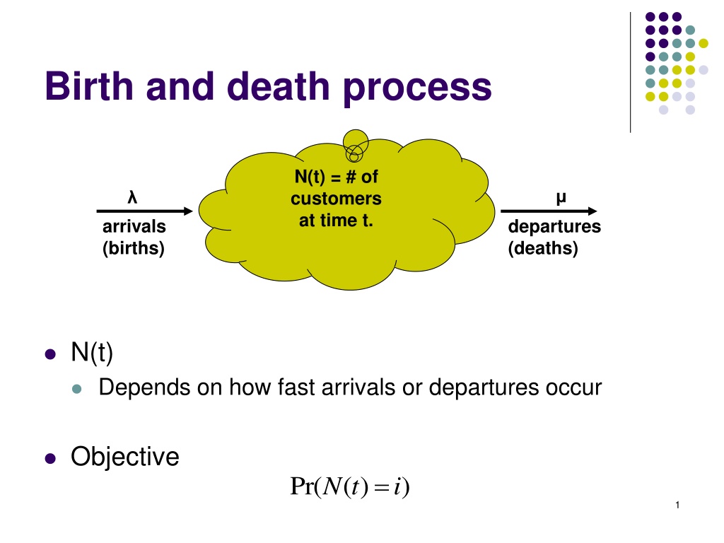
Depends on how fast arrivals or departures occur
Objective

N
(
t
)
=
#
o
f
c
u
s
t
o
m
e
r
s
a
t
t
i
m
e
t
.

λ
a
r
r
i
v
a
l
s
(
b
i
r
t
h
s
)

d
e
p
a
r
t
u
r
e
s
(
d
e
a
t
h
s
)
μ


2
B
e
h
a
v
i
o
r
o
f
t
h
e
s
y
s
t
e
m
λ
>
μ
λ
<
μ
Possible evolution of N(t)
Time


1 2 3 4 5 6 7 8 9 10 11


N
(
t
)
3
G
e
n
e
r
a
l
a
r
r
i
v
a
l
a
n
d
d
e
p
a
r
t
u
r
e
r
a
t
e
s
λ
n
Depends on the number of customers (n) in the system
Example
μ
n
Depends on the number of customers in the system
Example
4
C
h
a
n
g
i
n
g
t
h
e
s
c
a
l
e
o
f
a
u
n
i
t
t
i
m
e
Number of arrivals/unit time
Follows the Poisson distribution with rate
λ
n
Inter-arrival time of successive arrivals
is exponentially distributed
Average inter-arrival time = 1/
λ
n
What is the avg. # of customers arriving in dt?
T
i
m
e
5
P
r
o
b
a
b
i
l
i
t
y
o
f
o
n
e
a
r
r
i
v
a
l
i
n
d
t
dt so small
Number of arrivals in dt, X is a r.v.
X=1 with probability p
X=0 with probability 1-p
Average number of arrivals in dt
Prob (having one arrival in dt) =
λ
n
dt
dt
6
P
r
o
b
a
b
i
l
i
t
y
o
f
h
a
v
i
n
g
2
e
v
e
n
t
s
i
n
d
t
Departure rate in dt
μ
n
dt
Arrival rate in dt
λ
n
dt
What is the probability
Of having an (arrival+departure), (2 arrivals or departures)
7
P
r
o
b
a
b
i
l
i
t
y
d
i
s
t
r
i
b
u
t
i
o
n
o
f
N
(
t
)
P
n
(t)
The probability of getting n customers by time t
The distribution of the # of customers in system
t+dt
t
?
n
n-1: arrival
n+1: departure
n: none of the above
8
D
i
f
f
e
r
e
n
t
i
a
l
e
q
u
a
t
i
o
n
m
o
n
i
t
o
r
i
n
g
e
v
o
l
u
t
i
o
n
o
f
#
c
u
s
t
o
m
e
r
s
These are solved
Numerically using MATLAB
We will explore the cases
Of pure death
And pure birth
9
P
u
r
e
b
i
r
t
h
p
r
o
c
e
s
s
In this case
μ
n
=0, n >= 0
λ
n
=
λ
, n >= 0
Hence,
F
i
r
s
t
o
r
d
e
r
d
i
f
f
e
r
e
n
t
i
a
l
e
q
u
a
t
i
o
n
10
11
P
u
r
e
d
e
a
t
h
p
r
o
c
e
s
s
In this case
λ
n
=0, n >= 0
μ
n
=
μ
12
Q
u
e
u
i
n
g
s
y
s
t
e
m
Transient phase
Steady state
Behavior is independent of t
P
n
(t)
λ
μ
P
n
(t)
t
transient
Steady state
13
D
i
f
f
e
r
e
n
t
i
a
l
e
q
u
a
t
i
o
n
:
s
t
e
a
d
y
s
t
a
t
e
a
n
a
l
y
s
i
s
Limiting case
14
S
o
l
v
i
n
g
t
h
e
e
q
u
a
t
i
o
n
s
n=1
n=2
(
1
)
(
1
)
=
>
15
P
n
What about P
0
16
N
o
r
m
a
l
i
z
a
t
i
o
n
e
q
u
a
t
i
o
n
17
C
o
n
d
i
t
i
o
n
a
l
p
r
o
b
a
b
i
l
i
t
y
a
n
d
c
o
n
d
i
t
i
o
n
a
l
e
x
p
e
c
t
a
t
i
o
n
:
d
.
r
.
v
.
X and Y are discrete r.v.
Conditional probability mass function
Of X given that Y=y
Conditional expectation of X given that Y=y
18
C
o
n
d
i
t
i
o
n
a
l
p
r
o
b
a
b
i
l
i
t
y
a
n
d
e
x
p
e
c
t
a
t
i
o
n
:
c
o
n
t
i
n
u
o
u
s
r
.
v
.
If X and Y have a joint pdf
f
X,Y
(x,y)
Then, the
conditional probability density function
Of X given that Y=y
The conditional expectation
Of X given that Y=y
19
C
o
m
p
u
t
i
n
g
e
x
p
e
c
t
a
t
i
o
n
s
b
y
c
o
n
d
i
t
i
o
n
i
n
g
Denote
E[X|Y]
: function of the r.v. Y
Whose value at Y=y is E[X|Y=y]
E[X|Y]
: is itself a random variable
Property of conditional expectation
if Y is a discrete r.v.
if Y is continuous with density
f
Y
(y) =>
(
1
)
(
2
)
(
3
)
20
P
r
o
o
f
o
f
e
q
u
a
t
i
o
n
w
h
e
n
X
a
n
d
Y
a
r
e
d
i
s
c
r
e
t
e
21
P
r
o
b
l
e
m
1
Sam will read
Either one chapter of his probability book or
One chapter of his history book
If the number of misprints in a chapter
Of his probability book
is Poisson distributed with mean 2
Of his history book
is Poisson distributed with mean 5
Assuming Sam equally likely to choose either book
What is the expected number of misprints he comes across?
22
S
o
l
u
t
i
o
n
23
P
r
o
b
l
e
m
2
A miner is trapped in a mine containing three doors
First door
leads to a tunnel that takes him to safety
After 2 hours of travel
Second door
leads to a tunnel that returns him to the mine
After 3 hours of travel
Third door
Leads to a tunnel that returns him to the mine
After 5 hours
Assuming he is equally likely to choose any door
What is the expected length of time until he reaches
safety?
24
S
o
l
u
t
i
o
n
25
C
o
m
p
u
t
i
n
g
p
r
o
b
a
b
i
l
i
t
i
e
s
b
y
c
o
n
d
i
t
i
o
n
i
n
g
Let E denote an arbitrary event
X is a random variable defined by
It follows from the definition of X
26
P
r
o
b
l
e
m
3
Suppose that the number of people
Who visit a yoga studio each day
is a Poisson random variable with mean
λ
Suppose further that each person who visit
is, independently, female with probability p
Or male with probability 1-p
Find the joint probability
That n women and m men visit the academy today
27
S
o
l
u
t
i
o
n
Let
N
1
denote the number of women, N
2
the number of men
Who visit the academy today
N= N
1
+N
2
: total number of people who visit
Conditioning on N gives
Because P(N1=n,N2=m|N=i)=0 when i != n+m
28
S
o
l
u
t
i
o
n
(
c
o
n
t
’
d
)
Each of the n+m visit
is independently a woman with probability p
The conditional probability
That n of them are women is
The binomial probability of n successes in n+m trials
29
S
o
l
u
t
i
o
n
:
a
n
a
l
y
s
i
s
When each of a Poisson number of events
is independently classified
As either being type 1 with probability p
Or type 2 with probability (1-p)
=> the numbers of type 1 and 2 events
Are independent Poisson random variables
30
P
r
o
b
l
e
m
4
At a party
N men take off their hats
The hats are then mixed up and
Each man randomly selects one
A match occurs if a man selects his own hat
What is the probability of no matches?
31
S
o
l
u
t
i
o
n
E = event that no matches occur
P(E) = P
n
: explicit dependence on n
Start by conditioning
Whether or not the first man selects his own hat
M: if he did, M
c
: if he didn’t
P(E|M
c
)
Probability no matches when n-1 men select of n-1
That does not contain the hat of one of these men
32
S
o
l
u
t
i
o
n
(
c
o
n
t
’
d
)
P(E|M
c
)
Either there are no matches and
Extra man does not select the extra hat
=> P
n-1
(as if the extra hat belongs to this man)
Or there are no matches
Extra man does select the extra hat
=> (1/n-1)xP
n-2
33
S
o
l
u
t
i
o
n
(
c
o
n
t
’
d
)
P
n
is the probability of no matches
When n men select among their own hats
=> P
1
=0 and P
2
= ½
=>
34
P
r
o
b
l
e
m
5
:
c
o
n
t
i
n
u
o
u
s
r
a
n
d
o
m
v
a
r
i
a
b
l
e
s
The probability density function of a non-negative
random variable X is given by
Compute the constant
λ
?
35
P
r
o
b
l
e
m
6
:
c
o
n
t
i
n
u
o
u
s
r
a
n
d
o
m
v
a
r
i
a
b
l
e
s
Buses arrives at a specified stop at 15 min intervals
Starting at 7:00 AM
They arrive at 7:00, 7:15, 7:30, 7:45
If the passenger arrives at the stop at a time
Uniformly distributed between 7:00 and 7:30
Find the probability that he waits less than 5 min?
Solution
Let X denote the number of minutes past 7
That the passenger arrives at the stop
=>X is uniformly distributed over (0, 30)
36
P
r
o
b
l
e
m
7
:
c
o
n
d
i
t
i
o
n
a
l
p
r
o
b
a
b
i
l
i
t
y
Suppose that p(x,y) the joint probability mass
function of X and Y is given by
P(0,0) = .4, P(0,1) = .2, P(1,0) = .1, P(1,1) = .3
Calculate the conditional probability mass function of
X given Y = 1
37
c
o
u
n
t
i
n
g
p
r
o
c
e
s
s
A stochastic process {N(t), t>=0}
is said to be a counting process if
N(t) represents the total number of events that occur by time t
N(t) must satisfy
N(t) >= 0
N(t) is integer valued
If s < t, then N(s) <= N(t)
For s < t, N(s) – N(t) = # events in the interval (s,t]
Independent increments
# of events in disjoint time intervals are independent
38
P
o
i
s
s
o
n
p
r
o
c
e
s
s
The counting process {N(t), t>=0} is
Said to be a Poisson process having rate
λ
, if
N(0) = 0
The process has independent increments
The # of events in any interval of length t is
Poisson distributed with mean
λ
t, that is
39
P
r
o
p
e
r
t
i
e
s
o
f
t
h
e
P
o
i
s
s
o
n
p
r
o
c
e
s
s
Superposition property
If k independent Poisson processes
A1, A2, …, An
Are combined into a single process A
=> A is still Poisson with rate
Equal to the sum of individual
λ
i of Ai
40
P
r
o
p
e
r
t
i
e
s
o
f
t
h
e
P
o
i
s
s
o
n
p
r
o
c
e
s
s
(
c
o
n
t
’
d
)
Decomposition property
Just the reverse process
“A” is a Poisson process split into n processes
Using probability Pi
The other processes are Poisson
With rate Pi.
λ
Lambda = rate at which customers arrive = average # of arrivals per unit time. Mu = rate at which the customers depart.
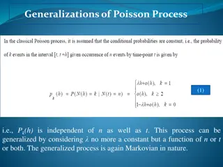
Explore the dynamics of birth and death processes in queueing systems, where the number of customers changes over time due to arrivals and departures. Learn about the behavior of systems, general arrival and departure rates, and the probability of events within given time intervals. Discover the probability distribution of the number of customers at any given time and delve into the differential equations governing customer evolution. Numerical solutions using MATLAB provide insights into this intriguing system.

Uploaded on Feb 26, 2025 | 0 Views
Download Presentation

Please find below an Image/Link to download the presentation.
The content on the website is provided AS IS for your information and personal use only. It may not be sold, licensed, or shared on other websites without obtaining consent from the author.If you encounter any issues during the download, it is possible that the publisher has removed the file from their server.
You are allowed to download the files provided on this website for personal or commercial use, subject to the condition that they are used lawfully. All files are the property of their respective owners.
The content on the website is provided AS IS for your information and personal use only. It may not be sold, licensed, or shared on other websites without obtaining consent from the author.
E N D
Presentation Transcript
Birth and death process N(t) = # of customers at time t. arrivals (births) departures (deaths) N(t) Depends on how fast arrivals or departures occur Objective = Pr( ( ) ) N t i 1
Behavior of the system > < Possible evolution of N(t) N(t) busy idle 3 2 1 1 2 3 4 5 6 7 8 9 10 11 2 Time
General arrival and departure rates n Depends on the number of customers (n) in the system Example , n M = n = , 0 n M n Depends on the number of customers in the system = n n Or Example = 3 n n
Changing the scale of a unit time Time Number of arrivals/unit time Follows the Poisson distribution with rate n Inter-arrival time of successive arrivals is exponentially distributed Average inter-arrival time = 1/ n What is the avg. # of customers arriving in dt? = hour Example n Average dt n 4 = = . 0 / 1 = : 30 / 30 16 / min 2 / min
Probability of one arrival in dt dt so small Number of arrivals in dt, X is a r.v. X=1 with probability p dt X=0 with probability 1-p Average number of arrivals in dt X E , = [ + n = [ ] . 1 0 .( 1 ) p p p = = ] but E X dt Prob (having one arrival in dt) = n dt 5
Probability of having 2 events in dt Departure rate in dt n dt Arrival rate in dt n dt What is the probability Of having an (arrival+departure), (2 arrivals or departures) ) 1 1 Pr( departure arrival = + = = 2 . ( ) dt dt dt n n n n 2 = = 2 2 Pr( 2 ) ( ) ( ) arrivals dt dt n n = 6 2 2 2 Pr( 2 ) ( ) ( ) departures dt dt n n
Probability distribution of N(t) Pn (t) The probability of getting n customers by time t The distribution of the # of customers in system t+dt t ? n n-1: arrival n+1: departure n: none of the above + = + ( P ) ( ) ( ) P + t dt P t dt P t dt + + 1 1 1 1 n n n n n ( )( 1 ) t dt dt n n n 7
Differential equation monitoring evolution of # customers + = + t P dt t P n + ( ) ( ) ( ) ( )( 1 ) P t dt P t dt P t dt P t dt dt + + 1 1 1 1 n n n n n n n n + ( ) ( ) n = + + ( ) ( ) ( )( ) n P t P t P t + + 1 1 1 1 n n n n n n dt P = + + ' ( = ) ( ) ( ) ( )( ) P t P t P t P t + + 1 1 1 1 n n n n n n n n ( ) ? t n These are solved Numerically using MATLAB We will explore the cases Of pure death And pure birth 8
Pure birth process In this case n =0, n >= 0 n = , n >= 0 = ' ( ) ( ) ( ) , 0 P t P t P t n Hence, = 1 n n n = ' ( ) . ( ), 0 P t P t n 0 0 t = ' ( ) ( ) ( ) , 0 P t P P t n 1 n n n n t ( ) t e = = t ( ) ; ( ) P t e P t 0 n ! n 9
First order differential equation ? ? + ? ? ? ? = ? ? y t ? ? ? ??+ ? ? ? ??? ? ? ? = ? ? ? ? ? ?? ? ?(?)? ? ? ??= ? ? ? ? ? ?? ? ? ? ? ? ??= ? ? ? ? ? ???? + ? ? ? = ? ? ? ?? ? ? ? ? ? ???? + ? ????? ? ?? ? ? = ?,? ? = ??? ,??? ? ? = ?? 1? ??? = ? ?? ?? 1(?) ? ???? + ? 10
Pure death process In this case n =0, n >= 0 n = = ' ( ) ( ) ( ) , 0 P t P t P t n + 1 n n n = ' ( ) ( ) ( = ) , 0 P t P t P t n + 1 n n n = ' ( ) . ( ), P t P t n M M M M n t ( ) t e = = t ( ) ; ( ) P t e P t M n ( )! M n 11
Queuing system Transient phase Pn (t) Steady state transient Steady state Behavior is independent of t Pn (t) t lim = ( ) P t P n n 12 t
Differential equation: steady state analysis Limiting case lim t = ( ) P t P n n lim t = ' ( ) 0 P t n = + + 0 ( ) , 0 P P P n + + 1 = 1 P 1 1 n n n n n n n P 0 0 + 1 ) 1 = + ( , 0 P P P n + + 1 1 1 1 n n n n n n n = 0 P P 1 0 1 13
Solving the equations n=1 + = + ( ) P P P (1) 1 1 1 0 0 2 2 n=2 + = + ( ) P P P 2 2 2 1 1 3 3 + = + P P P P (1) => 1 1 1 1 1 1 2 2 = = 1 P P P P 1 1 2 2 2 1 2 = 0 1 P P 2 0 1 2 14
Pn + = + P P P P 2 2 2 2 2 2 3 3 = = 2 P P P P 2 2 3 3 3 2 3 = 0 1 2 P P 2 0 1 2 3 ... = 0 1 1 , 1 n P P n 0 n ... 1 2 n What about P0 15
Normalization equation + + + ion + = ... .... 1 P P P 0 1 n Normilizat + + + = 0 0 1 .... 1 P P P 0 0 0 1 1 2 1 = P 0 1 n = n i = n + 1 0 i = i 1 i 1 16
Conditional probability and conditional expectation: d.r.v. X and Y are discrete r.v. Conditional probability mass function Of X given that Y=y | ( | X P = = = = = ) ( | ) p x y P X x Y y X Y = ( , ) ( , ) x Y y p x y = = ( ) ( ) P Y y p y Y Conditional expectation of X given that Y=y x = = = = [ | ] P . ( | ) E X Y y x X x Y y 17
Conditional probability and expectation: continuous r.v. If X and Y have a joint pdf fX,Y(x,y) Then, the conditional probability density function Of X given that Y=y ( , ) f x y = ( | ) f x y | X Y ( ) f y Y The conditional expectation Of X given that Y=y + = = [ | ] . ( | ) E X Y y x f x y dx Y | X 18
Computing expectations by conditioning Denote E[X|Y]: function of the r.v. Y Whose value at Y=y is E[X|Y=y] E[X|Y]: is itself a random variable Property of conditional expectation [ E = ] [ [ | ]] X E E X Y (1) if Y is a discrete r.v. = X E ] [ y = = = [ [ | ]] [ | ]. [ ] E E X Y E X Y y P Y y (2) if Y is continuous with density fY (y) => = X E ] [ + = [ | ] ( ) E X Y y f y dy (3) Y 19
Proof of equation when X and Y are discrete = = = [ [ | ]] [ | ]. [ ] E E X Y E X Y y P Y y y = = = = [ | ]. [ ] xP X x Y y P Y y y x = = [ , ] P X x Y y = = [ ] x P Y y = [ ] P Y y = y x = = = = = [ , ] [ , ] xP X x Y y x P X x Y y y x x y = = = [ ] [ ] xP X x E X x 20
Problem 1 Sam will read Either one chapter of his probability book or One chapter of his history book If the number of misprints in a chapter Of his probability book is Poisson distributed with mean 2 Of his history book is Poisson distributed with mean 5 Assuming Sam equally likely to choose either book What is the expected number of misprints he comes across? 21
Solution = _ X number mistakes , 1 _ _ chosen history book chosen = Y , 2 = _ probabilit y = ] 1 = + = = [ ] [ | 1 ]. [ [ | 2 ]. [ ] 2 E X E X Y P Y E X Y P Y 1 1 7 = + = ( 5 ) ( 2 ) 2 2 2 22
Problem 2 A miner is trapped in a mine containing three doors First door leads to a tunnel that takes him to safety After 2 hours of travel Second door leads to a tunnel that returns him to the mine After 3 hours of travel Third door Leads to a tunnel that returns him to the mine After 5 hours Assuming he is equally likely to choose any door What is the expected length of time until he reaches safety? 23
Solution = Y _ _ X time until safety = X _ _ P door initially chosen = = ] 1 = + = = [ E ] X [ | ] 1 = Y [ [ | ] 2 [ ] 2 E E X Y Y E X Y P Y + = = [ | ] 3 [ ] 3 Y P 1 ] 1 = + = + = ( [ | [ | ] 2 [ | 3 ]) E X Y E X Y E X Y 3 = = = = + [ | ) 1 = ; 2 [ E | ] 2 3 [ ]; E X Y E X Y E X = + [ | ] 3 5 [ ] E X Y X 1 = + + + + = [ ] 2 ( 3 3 [ ] 5 [ ] [ ] 10 E X E X E X E X 24
Computing probabilities by conditioning Let E denote an arbitrary event X is a random variable defined by = if _ , 0 , 1 _ _ if E occurs X _ ' E doesn t It follows from the definition of X = = = = [ ] ( ) [ | ] ( | ) E ) 2 ( X & P E E X Y y P E Y y ) 3 ( y = = = ( ) ( | ). ( , ) _ P E P E Y y P Y y Y discrete + = = ( ) ( | ) ( ) , _ P E P E Y y f y dy Y continuous 25 Y
Problem 3 Suppose that the number of people Who visit a yoga studio each day is a Poisson random variable with mean Suppose further that each person who visit is, independently, female with probability p Or male with probability 1-p Find the joint probability That n women and m men visit the academy today 26
Solution Let N1 denote the number of women, N2 the number of men Who visit the academy today N= N1 +N2 : total number of people who visit Conditioning on N gives 0 = = = = = = = ( , ) ( , | ). ( ) P N n N m P N n N m N i P N i 1 2 1 2 Because P(N1=n,N2=m|N=i)=0 when i != n+m = = = = = = + = + ( , ) ( , | ). ( ) P N n N m P N n N m N n m P N n m 1 2 1 2 + n m = = = = + ( , | ). P N n N m N n m e 1 2 + ( )! n m 27
Solution (contd) Each of the n+m visit is independently a woman with probability p The conditional probability That n of them are women is The binomial probability of n successes in n+m trials n m N n N P + + m n m = = = n m ( , ) 1 ( ) p p e 1 2 + n ( )! n m n m ( ) ( 1 ( )) p p = 1 ( ) p p e e ! ! n m 28
Solution: analysis n ( ) p = = = = = p ( ) ( , ) P N n P N n N m e 1 1 2 ! n = 0 m and m ( 1 ( )) p = = 1 ( ) p ( ) P N m e 2 ! m When each of a Poisson number of events is independently classified As either being type 1 with probability p Or type 2 with probability (1-p) => the numbers of type 1 and 2 events Are independent Poisson random variables 29
Problem 4 At a party N men take off their hats The hats are then mixed up and Each man randomly selects one A match occurs if a man selects his own hat What is the probability of no matches? 30
Solution E = event that no matches occur P(E) = Pn : explicit dependence on n Start by conditioning Whether or not the first man selects his own hat M: if he did, Mc : if he didn t M E P E P P n ) | ( ) ( = = + c c ( ) ( | ) ( ); P M P E M 1 P M n = = c ( | ) 0 ( | ) P E M P P E M n n P(E|Mc) Probability no matches when n-1 men select of n-1 That does not contain the hat of one of these men 31
Solution (contd) P(E|Mc) Either there are no matches and Extra man does not select the extra hat => Pn-1 (as if the extra hat belongs to this man) Or there are no matches Extra man does select the extra hat 1 = + c ( | ) P E M P P => (1/n-1)xPn-2 1 2 n n 1 n n 1 1 n n = + P P P 1 2 n n n 32
Solution (contd) Pn is the probability of no matches When n men select among their own hats => P1 =0 and P2 = => 1 1 1 1 1 = = + ; P P 3 4 ! 2 ! 3 ! 2 ! 3 ! 4 n 1 1 1 ( ) 1 n = + + .... P n ! 2 ! 3 ! 4 ! 33
Problem 5: continuous random variables The probability density function of a non-negative random variable X is given by x = ( ) . f x e 10 X Compute the constant ? + = = / 10 x 1 ( ) f x dx e dx X 0 1 = = = / 10 x 1 10 ( ). 10 e 10 0 34
Problem 6: continuous random variables Buses arrives at a specified stop at 15 min intervals Starting at 7:00 AM They arrive at 7:00, 7:15, 7:30, 7:45 If the passenger arrives at the stop at a time Uniformly distributed between 7:00 and 7:30 Find the probability that he waits less than 5 min? Solution Let X denote the number of minutes past 7 That the passenger arrives at the stop =>X is uniformly distributed over (0, 30) ) 15 10 Pr( + X = Pr( 25 30 ) X 15 30 1 1 1 + = dx dx 35 30 30 3 10 25
Problem 7: conditional probability ( | X P = = = = | ) ( | ) p x y P X x Y y X Y = = ( , ) ( , ) x Y y p x y = = ( ) ( ) P Y y p y Y Suppose that p(x,y) the joint probability mass function of X and Y is given by P(0,0) = .4, P(0,1) = .2, P(1,0) = .1, P(1,1) = .3 Calculate the conditional probability mass function of X given Y = 1 ) 1 ( = x = + = ( ) 1 , x ) 1 , 0 ( P ) 1 , 1 ( P 5 . 0 P P Y ) 1 , 0 ( P 2 = = , ) 1 | 0 ( Y hence P | X ) 1 ( Y P 5 ) 1 , 1 ( P 3 = = , ) 1 | 1 ( Y and P 36 | X ) 1 ( Y P 5
counting process A stochastic process {N(t), t>=0} is said to be a counting process if N(t) represents the total number of events that occur by time t N(t) must satisfy N(t) >= 0 N(t) is integer valued If s < t, then N(s) <= N(t) For s < t, N(s) N(t) = # events in the interval (s,t] Independent increments # of events in disjoint time intervals are independent 37
Poisson process The counting process {N(t), t>=0} is Said to be a Poisson process having rate , if N(0) = 0 The process has independent increments The # of events in any interval of length t is Poisson distributed with mean t, that is t n ( ) t + = = = ( ( ) ( ) ) , 1 , 0 ,... P N t s N s n e n ! n 38
Properties of the Poisson process Superposition property If k independent Poisson processes A1, A2, , An Are combined into a single process A => A is still Poisson with rate Equal to the sum of individual i of Ai 39
Properties of the Poisson process (cont d) Decomposition property Just the reverse process A is a Poisson process split into n processes Using probability Pi The other processes are Poisson With rate Pi. 40


")


")


")
")