Big Data Marketing Workshop
Prof. Taewan Kim from Konkuk University is conducting a Big Data Marketing Workshop focused on leveraging R for gaining customer insight. The workshop covers topics like data collection, text mining, data visualization, and managerial implications. Participants will learn about scraping data using rvest, utilizing Alexa for data manipulation, and installing necessary packages. Join to enhance your skills in Big Data Marketing Analytics!

Download Presentation

Please find below an Image/Link to download the presentation.
The content on the website is provided AS IS for your information and personal use only. It may not be sold, licensed, or shared on other websites without obtaining consent from the author.If you encounter any issues during the download, it is possible that the publisher has removed the file from their server.
You are allowed to download the files provided on this website for personal or commercial use, subject to the condition that they are used lawfully. All files are the property of their respective owners.
The content on the website is provided AS IS for your information and personal use only. It may not be sold, licensed, or shared on other websites without obtaining consent from the author.
E N D
Presentation Transcript
Big Data Marketing Big Data Marketing Workshop Workshop Getting the Customer Insight Using R Prof. Taewan Kim tkim21@konkuk.ac.kr
Prof. Taewan Kim Research Interests , , , , , , , Taewan Kim and Tridib Mazumdar, Product Concept Demonstrations in Trade Shows and Firm Value, Journal of Marketing, July 2016, Vol. 80, No. 4, pp. 90-108
Prof. Taewan Kim Teaching Interests ( ) ( ) (MBA) (MBA) Big Data Marketing Analytics ( ) ( )
Agenda What is Big Data? How can we collect Big Data? rvest.R Toolkit: SelectorGadget.com Exercise: alexa.r Text-mining tm.R Big Data Visualization Managerial implications Good example
R Download R: https://cloud.r-project.org/ Download R 4.1.2 for Windows (86 megabytes, 32/64 bit) Online resources (Feel free to utilize as much as you wish) RStudio: https://www.rstudio.com/products/rstudio/download/ Data Camp: https://www.datacamp.com/courses/free- introduction-to-r An Introduction to R would be good starting point. Manuals: https://cran.r-project.org/manuals.html
Rvest.R You need to install an extra gadget: http://selectorgadget.com/ Data scraping: http://blog.rstudio.org/2014/11/24/rvest-easy-web-scraping-with-r/ Alexa example (for, rbind, cbind): alexa.R html rvest : https://cran.r-project.org/web/packages/rvest/rvest.pdf Tutorial rvest: http://stat4701.github.io/edav/2015/04/02/rvest_tutorial/ Formatting data into table: https://cran.r- project.org/web/packages/data.table/vignettes/datatable-intro.pdf Scraping an HTML Table using rvest: http://www.r-bloggers.com/using- rvest-to-scrape-an-html-table/
echoshow10.r library(rvest) library(RCurl)
echoshow10.r # 1. Install two packages #install.packages('rvest') #install.packages('RCurl') library(rvest) library(RCurl)
echoshow10.r # 2. Identify the web address # search product - click reviews - sort by recent # remove the page number at the end of the URL url <- "https://www.amazon.com/All-new-Echo-Dot-3rd- Gen/product- reviews/B0792KTHKJ/ref=cm_cr_arp_d_viewopt_srt?ie=UTF8&re viewerType=all_reviews&sortBy=recent&pageNumber=" #url <- " your url "
echoshow10.r # 3. Specify how many pages you would like to scrape N_pages <- 3 # It would be easier to test with small number of pages and it depends on your own source website
echoshow10.r A <- NULL for (j in 1: N_pages){ echoshow <- read_html(paste0(url, j)) #help paste: http://www.cookbook- r.com/Strings/Creating_strings_from_variables/ B <- cbind(ipad %>% html_nodes(".review-text") %>% html_text(), echoshow10 %>% html_nodes("#cm_cr-review_list .review-date") %>% html_text() ) # I replaced html_nodes for review date with "#cm_cr-review_list .review-date" # "#cm_cr-review_list" makes two irrelevant parts for the top positive/critical reviews and '#'is the magic sign for unselect the part A <- rbind(A,B) }
echoshow10.r # 4. Make sure what you got print(j) # This command shows the progress of the for loop. This example it means number of pages. # 4.1 Another way to double-check tail(A,10) # 10 # 5. Save the output write.csv(data.frame(A),"echoshow10.csv")
tm.R Open this script file
#1. Installing relevant packages Needed <- c("tm", "SnowballCC", "RColorBrewer", "ggplot2", "wordcloud", "biclust", "cluster", "igraph", "fpc") install.packages(Needed, dependencies = TRUE) # install.packages("Rcampdf", repos = "http://datacube.wu.ac.at/", type = "source") #
#2. Loading texts 1. Save the collected data as CSV file 2. Move it into texts folder on the desktop 3. Change the code with your updated folder location Normally, you computer might have different folder location from the example code
#2.1 Change Folder and Directory cname <- file.path("C:/Users/user/Desktop", "texts") # This part should be revised by your own location of your texts folder. # Please make sure you exchange \ with /. Make sure you are using /. Also change your working directory
#3. Generating a Corpus # 3.0 Generating a Corpus, one document data set data <- read.csv( echoshow10.csv") #change the name of the file data<-data[,2] head(data) docs <- Corpus(VectorSource(data)) #summary(docs)
#3.1 Preprocessing # 3.1 Preprocessing ==parsing docs <- tm_map(docs,removePunctuation) docs <- tm_map(docs, removeNumbers) docs <- tm_map(docs, tolower) docs <- tm_map(docs, removeWords, stopwords("english")) docs <- tm_map(docs, removeWords, c("echo","show")) # you can add more irrelevant words hear! docs <- tm_map(docs, stripWhitespace)
#3.4 Word Frequency table ### 3.4 Plot Word Frequencies library(ggplot2) wf <- data.frame(word=names(freq), freq=freq) p <- ggplot(subset(wf, freq>200), aes(x = reorder(word, -freq), y = freq)) # Plot words that appear at least 200 times; You can modify this p <- p + geom_bar(stat="identity")+ theme(axis.text.x=element_text(angle=45, hjust=1)) p
750 500 freq 250 0 voicewellsee motionstill s good greatlikecan qualityonejustuse love much time evenset music works work homenew videowill reallyalso device kitchen reorder(word, -freq) cameraget devices follow room better sound amazon around picture feature product
#3.5 Word Association ### 3.5 Term Correlations # If words always appear together, then correlation=1.0. findAssocs(dtms, "great", corlimit=0.1) # specifying a correlation limit of 0.1 findAssocs(dtms, "quality", corlimit=0.1) # specifying a correlation limit of 0.1 findAssocs(dtms, "camera", corlimit=0.1) # specifying a correlation limit of 0.1
Word Association : clustering clue
#4. Word Clouds library(wordcloud) # First load the package that makes word clouds in R dtms <- removeSparseTerms(dtm, 0.9) # Prepare the data (max 10% empty space) freq <- colSums(as.matrix(dtm)) # Find word frequencies dark2 <- brewer.pal(6, "Dark2") # wordcloud(names(freq), freq, max.words=80) # wordcloud(names(freq), freq, min.freq=30, rot.per=0.4, colors=dark2) wordcloud(names(freq), freq, max.words=100, rot.per=0.2, colors=dark2)
watch something like s just make video will need get can nice family device little voice ask right using things easy firstlove awesome feature shows app house times motion call features everything speaker set smart camera buy product say home even cant dont think m lot day still want gen quality amazing devices back around work move display better follow one also sound works music every follows far time know thing best doesnt great amazon turn really good bought now support sometimes pretty room recipes well much picture seems always able use kitchen see new doesn t way used play
4. Word Clouds : , : :
#5.1 Hierarchical clustering ### 5.1 Hierarchal Clustering library(cluster) d <- dist(t(dtms), method="euclidian") # First calculate distance between words fit <- hclust(d=d, method="complete") # Also try: method="ward.D" plot.new() plot(fit, hang=-1) groups <- cutree(fit, k=5) # "k=" defines the number of clusters you are using rect.hclust(fit, k=5, border="red") # draw dendogram with red borders around the 8 clusters
#5.2 K-means clustering ### 5.2 K-means clustering #iteration, stopping rule library(fpc) library(cluster) dtms <- removeSparseTerms(dtm, 0.85) # Prepare the data (max 15% empty space) d <- dist(t(dtms), method="euclidian") kfit <- kmeans(d, 4) # set the clusters as 4 plot.new() op = par(mfrow = c(1, 1)) clusplot(as.matrix(d), kfit$cluster, color=T, shade=T, labels=2, lines=0)
Clustering word association (term correlation)
Recommendations review comments , Managerial implication
Good example How to leverage this text mining method