Bayes Models and Naive Bayes Algorithm Overview

Bayes Models

Outline
I. Naïve Bayes model
II. Revisiting the wumpus world
Lecture notes for
Principles of Artificial Intelligence
(COMS 4720/5720)
Yan-Bin Jia, Iowa State University

I. Naive Bayes Model

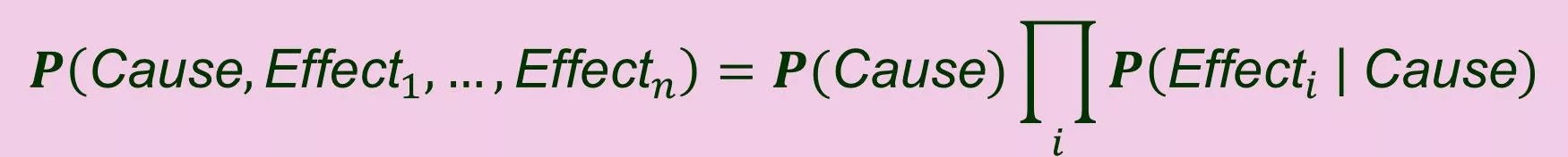

Full joint distribution:

Conditionally independent
given the cause
Hence the model is called “naïve”.
Inference
conditional independence of effects
When the effects are not conditionally independent:
(cont’d)
Take each possible cause.
Multiply its prior probability by the product of the conditional
probabilities of the observed effects given that cause.
Normalize the result
.
Calculate the probability distribution of the causes from observed effects:
Linear run time
in the number of observed effects only.
The
number of unobserved effects is irrelevant no matter how
large it is (as in medicine).
Text Classification
P
r
o
b
l
e
m
G
i
v
e
n
a
t
e
x
t
,
d
e
c
i
d
e
w
h
i
c
h
o
f
a
p
r
e
d
e
f
i
n
e
d
s
e
t
o
f
c
l
a
s
s
e
s
o
r
categories it belongs to.
{news, sports, business, weather, entertainment
}
Example sentences:
1.
Stocks rallied on Monday, with major indices gaining 1% as optimism persisted
over the first quarter earnings season.
2.
Heavy rain continued to pound much of the east coast on Monday, with flood
warnings issued in New York City and other locations.
Classify each sentence into a Category.
Classification (cont’d)
Classification Algorithm
Check which key words (i.e., effects) appear
.
Compute their posterior probability distribution over categories
(i.e. causes).
appearances/disappearances of the key words.
Other Applications of Naïve Bayes
Models
Language determination (
to detect the language a text is written in
)
Spam filtering (
to identify spam e-mails
)
Real-time prediction (
because they are very fast
)
Sentiment analysis (
to identify positive and negative customer sentiments
in social media)
Recommendation systems (
to filter unseen information and predict
whether a user would like a given resource or not
)
Medical diagnosis (
which requires more sophisticated models
)
Naïve Bayes models are not used in
II. The Wumpus World Revisited
Each of the three squares
might contain a pit.
Logical inference cannot conclude about
which square is most likely to be safe.
So a logical agent has no idea and has
to make a random choice.
A pit causes breeze in all neighboring squares.
Identify the set of random variables.
Full Joint Distribution
prior probability of
a pit configuration
Evidence
Q
u
e
r
y
// how likely does [1,3] contain a pit,
// given the observations so far?
Exponential in the number of squares!
Irrelevant Squares?
Outline
Frontier
: pit variables for the squares adjacent to visited ones.
Other
: pit variables for the other unknown squares.
10 other squares
I
n
s
i
g
h
t
:
T
h
e
o
b
s
e
r
v
e
d
b
r
e
e
z
e
s
a
r
e
c
o
n
d
i
t
i
o
n
a
l
l
y
independent of Other
, given
Known
,
Frontier
, and
the query variable.
Applying Conditional Independence
product rule
independent of
other
Elimination of Other Squares (
other
)
factoring
Probability of Containing a Pit
Delve into the principles of Artificial Intelligence with a study of Bayes models and the Naive Bayes algorithm. Understand the concepts of full joint distribution, conditional independence, and inference in Bayesian networks. Explore applications in text classification and learn about calculating probability distributions from observed effects. Experience a comprehensive overview of these essential topics for AI enthusiasts and students alike.

Download Presentation

Please find below an Image/Link to download the presentation.
The content on the website is provided AS IS for your information and personal use only. It may not be sold, licensed, or shared on other websites without obtaining consent from the author.If you encounter any issues during the download, it is possible that the publisher has removed the file from their server.
You are allowed to download the files provided on this website for personal or commercial use, subject to the condition that they are used lawfully. All files are the property of their respective owners.
The content on the website is provided AS IS for your information and personal use only. It may not be sold, licensed, or shared on other websites without obtaining consent from the author.
E N D
Presentation Transcript
Lecture notes for Principles of Artificial Intelligence (COMS 4720/5720) Yan-Bin Jia, Iowa State University Bayes Models Outline I. Na ve Bayes model II. Revisiting the wumpus world * Figures are from the textbook site.
I. Naive Bayes Model Full joint distribution: ? Cause,Effect1, ,Effect? = ?(Cause) ? Effect?Cause) ? Conditionally independent given the cause Often used in cases where the effect variables Effect1, ,Effect? are not strictly independent. Hence the model is called na ve .
Inference Observed effects: ? = ? Unobserved effects: ? = ? // ? = 1/?(?) = ??(Cause,?) ? Cause ?) conditional independence of effects ?(Cause,?,?) = ? ? ?? | Cause ? ? ? Cause ? ? Cause)? ? | Cause = ? ? = ?? Cause ? ??Cause) ? ? Cause) ? ? = 1 = ?? Cause ? ??Cause) ? When the effects are not conditionally independent: ? Cause ?) = ?? Cause ? ? |Cause
(contd) ? Cause ?) = ?? Cause ? ??Cause) ? Calculate the probability distribution of the causes from observed effects: Take each possible cause. Multiply its prior probability by the product of the conditional probabilities of the observed effects given that cause. Normalize the result. Linear run time in the number of observed effects only. Thenumber of unobserved effects is irrelevant no matter how large it is (as in medicine).
Text Classification Problem Given a text, decide which of a predefined set of classes or categories it belongs to. cause Category with range, e.g., {news, sports, business, weather, entertainment } effects HasWord?: presence or absence of the ?th keyword. Example sentences: 1. Stocks rallied on Monday, with major indices gaining 1% as optimism persisted over the first quarter earnings season. 2. Heavy rain continued to pound much of the east coast on Monday, with flood warnings issued in New York City and other locations. Classify each sentence into a Category.
Classification (contd) Prior probabilities: ?(Category) Conditional probabilities: ? HasWord?Category) ?(Category = ?) fraction of all previously seen documents that are of ?. ?(Category = weather) = 0.09 // 9% of articles are about weather. ? HasWord?Category) fraction of documents of each category that contain word ?. ? HasWord6= trueCategory = business) 0.37 // 37% of articles about business contain word 6, stocks .
Classification Algorithm Check which key words (i.e., effects) appear. Compute their posterior probability distribution over categories (i.e. causes). ? CategoryHasWord?) = ?? Category ? HasWord?Category) ? e.g., HasWords= HasWord1= true HasWord2= false appearances/disappearances of the key words.
Other Applications of Nave Bayes Models Language determination (to detect the language a text is written in) Spam filtering (to identify spam e-mails) Sentiment analysis (to identify positive and negative customer sentiments in social media) Real-time prediction (because they are very fast) Recommendation systems (to filter unseen information and predict whether a user would like a given resource or not) Na ve Bayes models are not used in Medical diagnosis (which requires more sophisticated models)
II. The Wumpus World Revisited Logical inference cannot conclude about which square is most likely to be safe. So a logical agent has no idea and has to make a random choice. We want to calculate the probability that each of squares [1,3],[2,2], and [3,1] contains a pit. A pit causes breeze in all neighboring squares. Each square other than [1,1] contains a pit with probability 0.2. Identify the set of random variables. ??,?: true if square [?,?] contains a pit. ??,?: true if square [?,?] is breezy included only for the observed squares, [1,1],[1,2],[2,1]. Each of the three squares might contain a pit.
Full Joint Distribution // ?1,1 false ? ?1,1, ,?4,4,?1,1,?1,2,?2,1 = ? ?1,1,?1,2,?2,1 | ?1,1, ,?4,4? ?1,1, ,?4,4 prior probability of a pit configuration values in the distribution, for a given pit configuration, are 1 if all the breezy squares among [1,1],[1,2],[2,1] are adjacent to pits, and 0 otherwise. 4,4 ? ?1,1, ,?4,4 = ?(??,?) ?,?=1,1 0.2? 0.815 ? for a configuration with ? 15 pits.
Evidence ? = ?1,1 ?1,2 ?2,1 known = ?1,1 ?1,2 ?2,1 ? ?1,3 | known, ? ? Query // how likely does [1,3] contain a pit, // given the observations so far? Unknown: a set of 12 ??,?s for squares other than the three known ones and the query one [1,3]. ? ?1,3 | known,? = ? ? ?1,3,known,?,unknown unknown { ?1,4,?2,2, ,?4,4, ,( ?1,4, ?2,2, ?4,4)} summation over 212= 4096 terms (if the full joint probabilities are available). Exponential in the number of squares!
Irrelevant Squares? Frontier: pit variables for the squares adjacent to visited ones. Outline [2,2] and [3,1] Other: pit variables for the other unknown squares. 10 other squares Unknown=Frontier Other Insight: The observed breezes are conditionally independent of Other, given Known, Frontier, and the query variable.
Applying Conditional Independence ? ?1,3,known,?,unknown {?1,4 ?2,2 ?4,4, , ?1,4 ?2,2 ?4,4} ? ?1,3 | known, ? = ? unknown product rule ? ? | ?1,3,known,unknown ? ?1,3,known,unknown = ? unknown ? ? | ?1,3,known,frontier,other ? ?1,3,known,frontier,other = ? other frontier ? is independent of other, given known, ?1,3, and frontier. ?2,2 ?3,1,?2,2 ?3,1, ?2,2 ?3,1, ?2,2 ?3,1 ? ? | ?1,3,known,frontier ? ?1,3,known,frontier,other = ? other frontier independent of other ? ? | ?1,3,known,frontier ? ?1,3,known,frontier,other = ? other frontier
Elimination of Other Squares (other) ? ?1,3 | known, ? ? ? | ?1,3,known,frontier ? ?1,3,known,frontier,other = ? other frontier factoring ? ? | ?1,3,known,frontier ? ?1,3?(known)?(frontier)?(other) = ? other frontier = ??(known)? ?1,3 ? ? | ?1,3,known,frontier ?(frontier) ?(other) other frontier ? =??(known)and ? other = 1 other ? ? | ?1,3,known,frontier ?(frontier) = ? ? ?1,3 frontier
Probability of Containing a Pit ? ?1,3 | known, ? = ? ? ?1,3 ? ? | ?1,3,known,frontier ?(frontier) frontier = 1 or 0 In the distribution ? ? | ?1,3,known,frontier : a probability is 1 if ? is consistent with the values of ?1,3 and the variables in frontier, and 0 otherwise. For each value of ?1,3, we sum over the logical models for the frontier variables that are consistent with known. ?1,3 ?1,3 Five consistent models for Frontier={?2,2,?3,1}: ? = ?1,1 ?1,2 ?2,1 known = ?1,1 ?1,2 ?2,1 ? ?1,3 | known, ? = ? 0.2 0.04 + 0.16 + 0.16 ,0.8(0.04 + 0.16) ?(?1,3) ? b | known, ?1,3 ? b | known, ?1,3 ?( ?1,3) 0.31,0.69 [1,3] contains a pit with 31% probability.


")

")


")