Automatic Picking of First Arrivals

 undefined
1
Automatic Picking of First Arrivals
He Dian and Ting Sun


Definition
•
The first-break picking
is that of identifying or
picking the first arrivals
of
refracted signals
from
all the signals received
by the receiver arrays
for a particular source
signal generation.
2
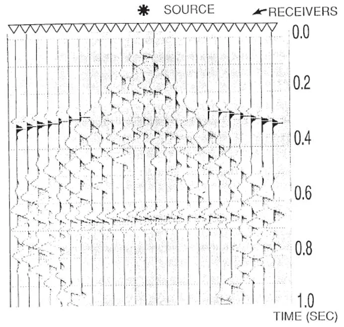
1.
Direct arrivals
2.
Reflected arrivals
3.
Refracted arrivals
3
•
One of the methods for studying the near-surface low-
velocity zone and for subsequent determination of static
corrections is the technique of employing
first arrivals
.
•
A common
static correction
is the weathering correction,
which compensates for a layer of low seismic velocity
material near the surface of the Earth.
Why?
5
6
7
Application
•
Static corrections for seismic data processing, an
important step in producing high-quality seismic
sections.
The weathering layer lead to near-surface low-velocity zone and
produces travel-time anomalies , and the anomalies result in false
subsurface structures in later seismic processing. However, the
anomalies can be corrected by using the first break arrival times on
refraction signals.
8
Application
•
Detailed knowledge of the structure of the low-velocity
zone.
9
Application
•
Used as observation data in reservoir history matching
History matching is the act of adjusting a model of a reservoir until it closely
reproduces the past behavior of a reservoir. The past behavior can be
production data and pressure data, well log and seismic data.
The accuracy of the history matching depends on the quality of the
reservoir model and the quality and quantity of observation data.
Once a model has been history matched, it can be used to simulate future
reservoir behavior with a higher degree of confidence.
10
The main difficulties are connected with the properties of
noise on seismograms:
1.
There is always a non-zero level of noise before first arrive.
2. The analysis of field data shows that first arrival and noise can be spatially
correlated over short distances.
3. Other anomalies in the topography of the survey region.
Difficulties
•
Coherence method.
•
Cross correlation method.
•
Combination of the correlation method an
linear least squares prediction technique.
•
Neural Networks.
•
Fractal-based algorithm.
2/18/2025
12
Methods
Automatic picking of first arrivals
•
Assume that the data of first arrivals are
presented by a seismogram
u
j,n
with
N
traces
recorded at points
x
n
=n
Δ
x, n=
1
, …, N
,
at time
moments
t
j
=j
Δ
t, j=
1
, …, J
.
13
Automatic picking of first arrivals
•
First step of the algorithm…
•
Destruction of a possible spatial correlation of noise.
•
This is achieved by suppression of noise with an
amplitude below a certain level.
•
This level is defined by estimation of the
average
maximum noise level
in a given time-space window
before the first arrivals.
14
Automatic picking of first arrivals
•
First step of the algorithm…
•
Let such a window be on the traces
m
1
to
m
2
•
For each trace
m
, the maximum noise level is defined,
•
Average maximum level of noise,
•
Define a unit step function,
•
The process of noise suppression is expressed as,
where
α
is a minimum threshold value of the ratio of the signal to the average
maximum noise level.
15
Automatic picking of first arrivals
•
Second step of the algorithm…
•
is first-arrival detection.
•
This is based on statistical estimates obtained by
summation of traces along straight lines in given
directions.
•
In order to define the directions of summation, we
introduce the dimensionless slowness:
where
Δ
x
is the distance between traces,
Δ
t
is the time sampling
interval and
v
k
is the apparent velocity in the direction of summation.
16
Automatic picking of first arrivals
•
Second step of the algorithm…
•
Define a range of summation over
L
traces, with
L
=2
L
H
+1 around the central trace
n
.
•
Then by summation in direction
P
k
, get the average,
•
And the standard deviation
•
Now introduce the function,
17
Automatic picking of first arrivals
•
Second step of the algorithm…
•
The function can serve as a good estimate for signal-
to-noise ratio, as can be clearly seen from two
extreme cases.
–
(1) absence of signal gives a very small value for
W
–
(2) ideal signal on all traces gives infinite value for
W
18
Automatic picking of first arrivals
•
Second step of the algorithm…
•
However, in practice we do not know the real distribution
of
U
and furthermore, we must deal with very small
ranges of summation.
•
Thus, propose the following criterion for signal detection
where assuming that on M traces (
M
<
L
) there are random deviations of noise
with the same amplitude
a
in a direction
P
k
. The noise is negligible on the
remaining
L-M
traces.
19
Automatic picking of first arrivals
•
Second step of the algorithm…
•
can serve as a measure of reliability of signal detection.
•
The inequality
is a criterion for making a decision regarding the
presence of a signal. This means that we eliminate the
possibility of false detection due to random correlation of
noise on
M
traces.
20
Automatic picking of first arrivals
•
Third step of the algorithm…
•
Find the time of first arrivals on trace
n
.
•
Average in a given time window
I
Δ
t
,
•
Next, for every value of
k
we find a minimum value of
j
, let it equal , for which the inequality
is satisfied.
21
Automatic picking of first arrivals
•
Third step of the algorithm…
•
In order to increase the reliability of detection, we
demand that this inequality is satisfied for several
consecutive values of in
j
.
•
Then, we find the minimum of all the values , let
it equal .
•
The value
thus is the estimate of the time of first arrivals on
trace
n
.
22
Thanks
Questions?
23
Identifying first arrivals of signals is crucial in seismic data processing to correct travel-time anomalies caused by near-surface low-velocity zones. This technique helps in studying the structure of these zones and improves the accuracy of reservoir history matching.

Download Presentation

Please find below an Image/Link to download the presentation.
The content on the website is provided AS IS for your information and personal use only. It may not be sold, licensed, or shared on other websites without obtaining consent from the author. Download presentation by click this link. If you encounter any issues during the download, it is possible that the publisher has removed the file from their server.
E N D
Presentation Transcript
Automatic Picking of First Arrivals He Dian and Ting Sun 1
Definition The first-break picking is that of identifying or picking the first arrivals of refracted signals from all the signals received by the receiver arrays for a particular source signal generation. 2
1. Direct arrivals 2. Reflected arrivals 3. Refracted arrivals 3
Why? One of the methods for studying the near-surface low- velocity zone and for subsequent determination of static corrections is the technique of employing first arrivals. A common static correction is the weathering correction, which compensates for a layer of low seismic velocity material near the surface of the Earth.
Application Static corrections for seismic data processing, an important step in producing high-quality seismic sections. The weathering layer lead to near-surface low-velocity zone and produces travel-time anomalies , and the anomalies result in false subsurface structures in later seismic processing. However, the anomalies can be corrected by using the first break arrival times on refraction signals. 8
Application Detailed knowledge of the structure of the low-velocity zone. 9
Application Used as observation data in reservoir history matching History matching is the act of adjusting a model of a reservoir until it closely reproduces the past behavior of a reservoir. The past behavior can be production data and pressure data, well log and seismic data. The accuracy of the history matching depends on the quality of the reservoir model and the quality and quantity of observation data. Once a model has been history matched, it can be used to simulate future reservoir behavior with a higher degree of confidence. 10
Difficulties The main difficulties are connected with the properties of noise on seismograms: 1. There is always a non-zero level of noise before first arrive. 2. The analysis of field data shows that first arrival and noise can be spatially correlated over short distances. 3. Other anomalies in the topography of the survey region.
Methods Coherence method. Cross correlation method. Combination of the correlation method an linear least squares prediction technique. Neural Networks. Fractal-based algorithm. 2/18/2025 12
Automatic picking of first arrivals Assume that the data of first arrivals are presented by a seismogram uj,n with N traces recorded at points xn=n x, n=1, , N, at time momentstj=j t, j=1, , J. 13
Automatic picking of first arrivals First step of the algorithm Destruction of a possible spatial correlation of noise. This is achieved by suppression of noise with an amplitude below a certain level. This level is defined by estimation of the average maximum noise level in a given time-space window before the first arrivals. 14
Automatic picking of first arrivals First step of the algorithm Let such a window be on the traces m1 to m2 For each trace m, the maximum noise level is defined, Average maximum level of noise, Define a unit step function, The process of noise suppression is expressed as, where is a minimum threshold value of the ratio of the signal to the average maximum noise level. 15
Automatic picking of first arrivals Second step of the algorithm is first-arrival detection. This is based on statistical estimates obtained by summation of traces along straight lines in given directions. In order to define the directions of summation, we introduce the dimensionless slowness: where x is the distance between traces, t is the time sampling interval and vk is the apparent velocity in the direction of summation. 16
Automatic picking of first arrivals Second step of the algorithm Define a range of summation over L traces, with L=2LH+1 around the central trace n. Then by summation in direction Pk, get the average, And the standard deviation Now introduce the function, 17
Automatic picking of first arrivals Second step of the algorithm The function can serve as a good estimate for signal- to-noise ratio, as can be clearly seen from two extreme cases. (1) absence of signal gives a very small value for W (2) ideal signal on all traces gives infinite value for W 18
Automatic picking of first arrivals Second step of the algorithm However, in practice we do not know the real distribution of U and furthermore, we must deal with very small ranges of summation. Thus, propose the following criterion for signal detection where assuming that on M traces (M<L) there are random deviations of noise with the same amplitude a in a direction Pk. The noise is negligible on the remaining L-M traces. 19
Automatic picking of first arrivals Second step of the algorithm can serve as a measure of reliability of signal detection. The inequality is a criterion for making a decision regarding the presence of a signal. This means that we eliminate the possibility of false detection due to random correlation of noise on M traces. 20
Automatic picking of first arrivals Third step of the algorithm Find the time of first arrivals on trace n. Average in a given time window I t, Next, for every value of k we find a minimum value of j, let it equal , for which the inequality is satisfied. 21
Automatic picking of first arrivals Third step of the algorithm In order to increase the reliability of detection, we demand that this inequality is satisfied for several consecutive values of in j. Then, we find the minimum of all the values , let it equal . The value thus is the estimate of the time of first arrivals on trace n. 22
Thanks Questions? 23