Automated Quantification of 1D NMR Spectra with SAND
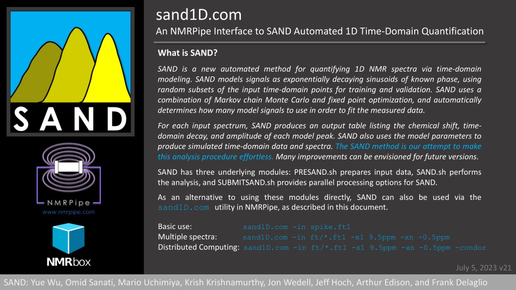
SAND is an automated method for quantifying 1D NMR spectra using time-domain modeling by modeling signals as exponentially decaying sinusoids. It uses random subsets of input data for training and validation, combining Markov chain Monte Carlo and fixed-point optimization. SAND determines the number of model signals needed to fit the data, producing output tables with peak information. It simplifies the analysis process and can be accessed via the sand1D.com utility. SAND is available on NMRbox for high-throughput computing.
Download Presentation

Please find below an Image/Link to download the presentation.
The content on the website is provided AS IS for your information and personal use only. It may not be sold, licensed, or shared on other websites without obtaining consent from the author.If you encounter any issues during the download, it is possible that the publisher has removed the file from their server.
You are allowed to download the files provided on this website for personal or commercial use, subject to the condition that they are used lawfully. All files are the property of their respective owners.
The content on the website is provided AS IS for your information and personal use only. It may not be sold, licensed, or shared on other websites without obtaining consent from the author.
E N D
Presentation Transcript
sand1D.com An NMRPipe Interface to SAND Automated 1D Time-Domain Quantification What is SAND? SAND is a new automated method for quantifying 1D NMR spectra via time-domain modeling. SAND models signals as exponentially decaying sinusoids of known phase, using random subsets of the input time-domain points for training and validation. SAND uses a combination of Markov chain Monte Carlo and fixed point optimization, and automatically determines how many model signals to use in order to fit the measured data. For each input spectrum, SAND produces an output table listing the chemical shift, time- domain decay, and amplitude of each model peak. SAND also uses the model parameters to produce simulated time-domain data and spectra. The SAND method is our attempt to make this analysis procedure effortless. Many improvements can be envisioned for future versions. SAND has three underlying modules: PRESAND.sh prepares input data, SAND.sh performs the analysis, and SUBMITSAND.sh provides parallel processing options for SAND. As an alternative to using these modules directly, SAND can also be used via the sand1D.com utility in NMRPipe, as described in this document. Basic use: sand1D.com -in spike.ft1 Multiple spectra: sand1D.com -in ft/*.ft1 -x1 9.5ppm -xn -0.5ppm Distributed Computing: sand1D.com -in ft/*.ft1 -x1 9.5ppm -xn -0.5ppm -condor July 5, 2023 v21 SAND: Yue Wu, Omid Sanati, Mario Uchimiya, Krish Krishnamurthy, Jon Wedell, Jeff Hoch, Arthur Edison, and Frank Delaglio
sand1D.com An NMRPipe Interface to SAND Automated 1D Time-Domain Quantification Where is SAND? SAND is available on NMRbox, and is set up to use NMRbox high throughput distributed computing via HTCondor. https://nmrbox.nmrhub.org SAND Github https://github.com/edisonomics/SAND SAND Demo Data https://www.ibbr.umd.edu/nmrpipe/sand_demo1.tar This Slide Deck https://www.ibbr.umd.edu/nmrpipe/sand1D_demo1.pptx SAND: Yue Wu, Omid Sanati, Mario Uchimiya, Krish Krishnamurthy, Art Edison, and Frank Delaglio Feb 28, 2023 v14
sand1D.com An NMRPipe Interface to SAND Automated 1D Time-Domain Quantification What is sand1D.com? The SAND modules can be used with many possible workflows, requiring a very specific arrangement of input files. In order to streamline and simplify the use of SAND, an NMRPipe utility script sand1D.com is available. The sand1D.com utility takes a list of one or more NMRPipe-format 1D spectra as input, automatically creates the needed file structures for SAND, and then executes modules PRESAND.sh, SUBMITSAND.sh, and SAND.sh to perform the analysis. In practice, this means that SAND can be applied simply by listing one or more related input spectra and the desired region of interest, for example: sand1D.com in plasma.ft1 spike.ft1 x1 9.0ppm xn -0.5ppm SAND: Yue Wu, Omid Sanati, Mario Uchimiya, Krish Krishnamurthy, Jon Wedell, Jeff Hoch, Arthur Edison, and Frank Delaglio
sand1D.com An NMRPipe Interface to SAND Automated 1D Time-Domain Quantification Example Result of SAND Analysis sand1D.com -in 001.ft1 -x1 8.7ppm -xn 6.7ppm -simAll Measured Spectrum SAND Model SAND Model Peaks SAND: Yue Wu, Omid Sanati, Mario Uchimiya, Krish Krishnamurthy, Jon Wedell, Jeff Hoch, Arthur Edison, and Frank Delaglio
sand1D.com An NMRPipe Interface to SAND Automated 1D Time-Domain Quantification sand1D.com -in 001.ft1 -x1 2.75ppm -xn 2.45ppm -simAll Measured Spectrum SAND Model SAND CSV Output (Excerpt) index, freq_ppm, decay_hz, amplitude 17, 2.5639, 7.628, 3.0528e+00 18, 2.5433, 7.845, 9.3367e+01 19, 2.5389, 14.485, 1.4976e+01 20, 2.5317, 7.718, 3.1815e+00 21, 2.5175, 8.197, 7.4027e+01 22, 2.5125, 9.329, 7.9201e+00 23, 2.5057, 10.255, 6.8238e+00 21, 74.03 SAND Model Peaks Peak ID, Integral 18, 93.37 23, 6.82 22, 7.92 20, 3.18 19, 14.98 17, 3.05 SAND: Yue Wu, Omid Sanati, Mario Uchimiya, Krish Krishnamurthy, Jon Wedell, Jeff Hoch, Arthur Edison, and Frank Delaglio
sand1D.com An NMRPipe Interface to SAND Automated 1D Time-Domain Quantification Output of sand1D.com When sand1D.com is invoked, it will automatically create a directory for the various output files that will be produced. The directory name will have the form sand0001 sand0002 etc. For every input spectrum, the SAND master directory will contain a subdirectory sand_data/1sand_data/2 etc. These subdirectories will contain copies of each input spectrum, and the workspaces used directly by the SAND modules. When the SAND analysis completes, the master directory will contain the following subdirectories, each having one output file of analysis results for each input spectrum: sand0001/csv/*.csv sand0001/tab/*.tab sand0001/simFID/*.fid sand0001/sim/*.ft1 sand0001/src/*.txt CSV-format Tables of PPM, Decay, and Amplitude NMRPipe-format Peak Tables for Simulation NMRPipe-format Simulated Time-Domain Data NMRPipe-format Spectra from Simulated FIDs Text files containing the names of the original input spectra If the sand1D.com -simAll option is used, output will also include simulations for each model peak, with subdirectories 1, 2, etc. for each input spectrum (Note! The -simAll option takes a lot of disk space, only use it when needed). sand0001/simAllFID/1/*.fid sand0001/simAll/1/*.ft1 NMRPipe-format Simulated Time-Domain Data NMRPipe-format Spectra from Simulated FIDs SAND: Yue Wu, Omid Sanati, Mario Uchimiya, Krish Krishnamurthy, Jon Wedell, Jeff Hoch, Arthur Edison, and Frank Delaglio
sand1D.com An NMRPipe Interface to SAND Automated 1D Time-Domain Quantification The SAND Workspace Directories sand_data and SAND_last_run As noted previously, when sand1D.com is invoked, it will automatically create a master directory for the various output files that will be produced. The directory name will have the form sand0001 sand0002 etc. SAND will create subdirectories sand_data and SAND_last_run in the master directory. It is not strictly necessary to retain these subdirectories once the SAND calculation is finished, because the final SAND results are summarized in sand0001/csv sand0001/tab sand0001/sim etc., as described previously. These subdirectories will contain copies of each input spectrum, and the workspaces used directly by the SAND modules. When a SAND computation is finished, the sand_data/SAND directory will contain many intermediate results, including matlab figures and redundant versions of the final results. sand0001/sand_data/1/test.ft Copy of input spectrum 1. NMRPipe-format simulated time-domain data NMRPipe-format Spectra from simulated FID CSV-format signal table sand0001/sand_data/1/sim.fid sand0001/sand_data/1/sim.ft1 sand0001/sand_data/1/sim.csv sand0001/sand_data/1/sim.tab sand0001/sand_data/1/SAND/ NMRPipe-format peak table for simulation Contains SAND matlab files and intermediate results SAND: Yue Wu, Omid Sanati, Mario Uchimiya, Krish Krishnamurthy, Jon Wedell, Jeff Hoch, Arthur Edison, and Frank Delaglio
sand1D.com An NMRPipe Interface to SAND Automated 1D Time-Domain Quantification Using SAND via Distributed Computing TBD SAND: Yue Wu, Omid Sanati, Mario Uchimiya, Krish Krishnamurthy, Jon Wedell, Jeff Hoch, Arthur Edison, and Frank Delaglio
sand1D.com An NMRPipe Interface to SAND Automated 1D Time-Domain Quantification Guidelines for Preparing Input Spectra for sand1D.com (Important!) Acquire spectra with no first order phase correction when possible. Besides making autoprocessing more difficult, the need for first order phase correction generally means there will also be baseline distortions. When converting Bruker format data to NMRPipe-format, use options for Digital Oversampling Correction: During Conversion (bruker dmx/bruk2pipe -DMX). Use only exponential line broadening. SAND will model the spectrum as-is, retaining any line broadening applied. The decay values in the output tables produced by sand1D.com (sand0001/tab/*.tab and csv/*.csv) will be reduced by the amount of exponential line broadening applied. Process spectra with exactly one zero fill, rounded up to a power of two. Keep the full spectral range (i.e. do not extract a subset of the spectrum such as via EXT). Phase and baseline correct the spectrum as well as possible. Perform any needed chemical shift calibration before using SAND. For speed, analyze the smallest spectral range (sand1D.com -x1 ... -xn ...). SAND: Yue Wu, Omid Sanati, Mario Uchimiya, Krish Krishnamurthy, Jon Wedell, Jeff Hoch, Arthur Edison, and Frank Delaglio
sand1D.com An NMRPipe Interface to SAND Automated 1D Time-Domain Quantification Limitations of SAND This first release of SAND was developed and tuned primarily for high-resolution 1H metabolomics data. As a result, the default settings might not be ideal for other types of data. This first release of SAND requires phase-corrected spectra as input. SAND can tolerate some baseline distortion, but results will be best if the input spectra are baseline corrected to the extent possible. Likewise, simplifying or blanking the solvent region of the input spectrum might also be helpful. SAND is computationally intensive, and this first release is slow. A typical spectrum might take overnight to process. To accommodate this, SAND includes advanced high-throughput processing options so that a batch of spectra can be analyzed as quickly and easily as one spectrum. SAND: Yue Wu, Omid Sanati, Mario Uchimiya, Krish Krishnamurthy, Jon Wedell, Jeff Hoch, Arthur Edison, and Frank Delaglio
sand1D.com An NMRPipe Interface to SAND Automated 1D Time-Domain Quantification Demo Data for Use with SAND https://www.ibbr.umd.edu/nmrpipe/sand_demo1.tar This demo data is a urine spectral series, with varying spike-in amounts of a four-compound mixture plus DSS. The data includes a script all.com that performs all of the conversion and processing for the series. NMRPipe workflows for batch processing usually consist of a combination of general-purpose utilities used via customized scripts. The batch processing schemes often use a table of metadata as input. This table specifies the locations of the spectrometer data directories to be processed, and also specifies titles for each of the spectra. A typical batch processing workflow: Establish the metadata table that lists the spectral data to process (here, meta.tab ). Convert each spectrometer data set to NMRPipe format. Process each time-domain data set. Calibrate chemical shifts. Interpolate spectra to identical sizes and chemical shift ranges. This optional step prepares a spectral series for multivariate methods such as Principal Component Analysis (PCA) which compare spectra on a point-by-point basis. SAND: Yue Wu, Omid Sanati, Mario Uchimiya, Krish Krishnamurthy, Jon Wedell, Jeff Hoch, Arthur Edison, and Frank Delaglio
sand1D.com An NMRPipe Interface to SAND Automated 1D Time-Domain Quantification A Quick Demo of SAND on a Small Region of Two Spectra This example uses SAND with parameter settings intended to produce a demo result quickly. It takes roughly 15 min to complete. Start a C-shell, get and unpack the demo data in your home directory: csh cd wget https://www.ibbr.umd.edu/nmrpipe/sand_demo1.tar tar xvf sand_demo1.tar Go to the demo data directory, which also contains measured data directories 1 - 7: cd sand_demo1 Execute the batch processing scheme created for this data (creates output interp/*.ft1): all.com Inspect the resulting spectra if desired: specView.tcl -in interp/*.ft1 Execute SAND on spectra 001 and 002 (or use quick.com ): sand1D.com -in interp/001*.ft1 interp/002*.ft1 -x1 2.65ppm -xn 2.45ppm \ -simAll -sandArgs -s 3 View the SAND Result for Spectrum 001 Using the specView.tcl Utility Directly: specView.tcl -in interp/001*.ft1 sand0001/sim/0001.ft1 sand0001/simAll/1/*.ft1 View the SAND Result for Spectrum 002 Using the Demo Script showSand.com: showSand.com -specID 2 SAND: Yue Wu, Omid Sanati, Mario Uchimiya, Krish Krishnamurthy, Jon Wedell, Jeff Hoch, Arthur Edison, and Frank Delaglio
sand1D.com An NMRPipe Interface to SAND Automated 1D Time-Domain Quantification A Manual Example of SAND with One Spectrum (See Also: sand_demo1/1/all.com) Start a C-shell, get and unpack the demo data: csh cd wget https://www.ibbr.umd.edu/nmrpipe/sand_demo1.tar tar xvf sand_demo1.tar Go to input data 1 in the demo data: cd sand_demo1/1 Create and execute a format conversion script: bruker -dmx -AUTO fid.com Process the data and calibrate chemical shifts: basicFT1.com -xP0 Auto -xP1 0.0 xBASEARG POLY,auto,ord=1,window=2% ref1D.tcl -x1 0.1ppm -xn -0.1ppm -tab ref.tab -max Inspect the resulting spectrum: nmrDraw Execute SAND (takes hours): sand1D.com in test.ft1 -x1 8.7ppm -xn 6.7ppm -simAll View the Result: specView.tcl -in test.ft1 sand0001/sim/0001.ft1 sand0001/simAll/1/*.ft1 SAND: Yue Wu, Omid Sanati, Mario Uchimiya, Krish Krishnamurthy, Jon Wedell, Jeff Hoch, Arthur Edison, and Frank Delaglio
sand1D.com An NMRPipe Interface to SAND Automated 1D Time-Domain Quantification A Batch Processing Example (See Also: sand_demo1/all.com andsand_demo1/sand_batch.com) Start a C-shell, get and unpack the demo data in your home directory: csh cd wget https://www.ibbr.umd.edu/nmrpipe/sand_demo1.tar tar xvf sand_demo1.tar Go to the demo data directory, which also contains measured data directories 1 - 7: cd sand_demo1 Execute the batch processing scheme created for this data (creates output interp/*.ft1): all.com Inspect the resulting spectra if desired: specView.tcl -in interp/*.ft1 Execute SAND on Batch (takes hours NOTE: CONDOR OPTIONS NOT YET TESTED): sand1D.com in interp/*.ft1 -x1 9.5ppm -xn -0.5ppm -simAll -condor View the SAND Result for Spectrum 1 Using the specView.tcl Utility Directly: specView.tcl -in interp/001*.ft1 sand0001/sim/0001.ft1 sand0001/simAll/1/*.ft1 View the SAND Result for Spectrum 2 Using the Demo Script showSand.com: showDemo.com -sandID 1 -specID 2 SAND: Yue Wu, Omid Sanati, Mario Uchimiya, Krish Krishnamurthy, Jon Wedell, Jeff Hoch, Arthur Edison, and Frank Delaglio
sand1D.com An NMRPipe Interface to SAND Automated 1D Time-Domain Quantification A Note About NMRPipe Utilities NMRPipe is script based, and has numerous general purpose utilities. Some of these are executable programs, some are C-shell scripts, and some are TCL scripts that use NMRPipe s custom TCL/TK interpreter nmrWish . Workflows in NMRPipe commonly use a combination of general purpose utilities and scripts that are custom-made for a particular application or dataset. The various general purpose utilities of NMRPipe can be invoked from the command line with the -help option, which will list the usage notes and command-line options of the utility. For example, utility basicFT1.com generates processing scripts for 1D data. It has many options and default values, including default values for the input and output file names. The complete set of command-line options and usage notes can be listed using the -help option: basicFT1.com -help For example, this command, with no other options, will process using P0 autophase with defaults: input test.fid , output test.ft1 , one zero fill, and 1.0 Hz exponential: basicFT1.com -xP0 Auto This example applies exponential broaden 0.3 Hz, auto first-order baseline correction, and autophase performed in 0.1 degree steps with temporary first-order baseline correction: basicFT1.com -xP0 Auto -xELB 0.3 -xBASEARG POLY,auto,window=2%,ord=1 \ -apOrd 1 -apArgs apxP0Step=0.1 SAND: Yue Wu, Omid Sanati, Mario Uchimiya, Krish Krishnamurthy, Jon Wedell, Jeff Hoch, Arthur Edison, and Frank Delaglio
sand1D.com An NMRPipe Interface to SAND Automated 1D Time-Domain Quantification Processing Script Auto-Generated by basicFT1.com # # Generated by basicFT1.com Version 2022.340.15.42 # # basicFT1.com -in test.fid -out test.ft1 -xP0 Auto \ # -xP0 Auto -xP1 0.0 -xELB 0.3 -xBASEARG POLY,auto,window=2%,ord=1 \ # -apOrd 1 -apArgs apxP0Step=0.1,apx1=5%,apxn=95% # # Auto-phase determination; arguments duplicated later on the # basicAutoPhase.com command line ignored: nmrPrintf "Auto-Phase ...\n\n" set xP0 = (`basicAutoPhase.com -in test.fid -apxP0Step 0.1 -apx1 5% -apxn 95% \ -apxELB 0.3 -apxP1 0.0 -apOrd 1 -apWindow 2%`) nmrPrintf "Auto-Phase xP0: %.1f\n\n" $xP0 nmrPipe -in test.fid \ | nmrPipe -fn SP -off 0.5 -end 0.5 -pow 1 -elb 0.3 -glb 0.0 -c 0.5 \ | nmrPipe -fn ZF -zf 1 -auto \ | nmrPipe -fn FT \ | nmrPipe -fn PS -p0 $xP0 -p1 0.0 -di \ | nmrPipe -fn POLY -auto -window 2% -ord 1 \ -out test.ft1 -ov SAND: Yue Wu, Omid Sanati, Mario Uchimiya, Krish Krishnamurthy, Jon Wedell, Jeff Hoch, Arthur Edison, and Frank Delaglio
sand1D.com An NMRPipe Interface to SAND Automated 1D Time-Domain Quantification An Example Metadata Table for NMRPipe Batch Processing (See Also: sand_demo1/all.com) NMRPipe workflows for batch processing usually consist of a combination of general- purpose utilities used via customized scripts. These workflows are often organized via metadata specified in an NMRPipe-format table giving the list of spectrometer-format data directories to be processed, along with titles for each of the measurements. The titles can encode any details of interest about the spectra, as one or more fields separated by dash characters - . In the case of this spike-in series, the title encodes the urine volume, buffer volume, and spike-in volume used to create the sample. Here is the metadata for this demo: # # File meta.tab, metadata for spike-in urine series. # Required: INDEX DIR_NAME TITLE VARS INDEX DIR_NAME TITLE FORMAT %3d %10s %s 1 1 spike0-urine540ul-buf60ul-spike0ul 2 2 spike1-urine540ul-buf60ul-spike20ul 3 3 spike2-urine540ul-buf60ul-spike40ul 4 4 spike3-urine540ul-buf60ul-spike60ul 5 5 spike4-urine540ul-buf60ul-spike80ul 6 6 ref-d2o0ul-buf60ul-spike20ul 7 7 buf-d2o540ul-buf60ul-spike0ul SAND: Yue Wu, Omid Sanati, Mario Uchimiya, Krish Krishnamurthy, Jon Wedell, Jeff Hoch, Arthur Edison, and Frank Delaglio
sand1D.com An NMRPipe Interface to SAND Automated 1D Time-Domain Quantification NMRPipe Batch Processing Workflows (See Also: sand_demo1/all.com) As noted, NMRPipe workflows for batch processing usually consist of a combination of general-purpose utilities used via customized scripts. There will typically be customized scripts clean.com configured to delete any previous results, conv.com to convert all of the data listed in the metadata table to NMRPipe format, and proc.com that will process all of the time-domain data. These scripts are often re-used as-is for similar batches of data. Additional steps can include a script that applies DSS chemical shift calibration to all spectra, or a step that interpolates all spectra so that they have identical sizes and chemical shift ranges so that they can be used more easily with methods that compare spectra on a point-by-point basis, such as principal component analysis. # # Delete any previous results. # Conversion with compensation for digital oversampling. # Processing with zero-order auto phase, and auto first-order baseline correction. # Chemical shift reference by DSS signal. # Optional step, interpolate spectra to identical size and ppm range. clean.com conv.com -meta meta.tab -outDir fid -cmnd bruker -AUTO -dmx proc.com -meta meta.tab -outDir ft ref1D.com -in ft/*.ft1 -x1 0.1ppm -xn -0.1ppm interp1D.com -inDir ft -outDir interp -ref None SAND: Yue Wu, Omid Sanati, Mario Uchimiya, Krish Krishnamurthy, Jon Wedell, Jeff Hoch, Arthur Edison, and Frank Delaglio
sand1D.com An NMRPipe Interface to SAND Automated 1D Time-Domain Quantification sand1D.com help SAND 1D Spectral Decomposition (Script Version 2023.043.14.54). Y Wu, O Sanati, M Uchimiya, K Krishnamurthy, A Edison, and F Delaglio. Options: -in ftList [test.ft1] List of NMRPipe-format 1D Spectra. -sandDir sandDir [Auto] SAND Master Output Directory (Auto = sand0001 ...). -cores nCores [40] Number of Processing Cores for Command-Line Processing. Analysis Region (pts ppm hz %): -x1 x1 [3%] Start Location of Analysis Region. -xn xn [97%] End Location of Analysis Region. Options for Creation of NMRPipe Simulated Data (Default = Use Value from Input Data): -lb lb [Default] Exponential Broaden in Hz. -p0 p0 [Default] Zero Order Phase. -p1 p1 [Default] First Order Phase. -rescale Rescale SAND Results (Default). -norescale No Rescale of SAND Results. -sim Generate Simulations from SAND Results (Default). -nosim Do Not Generate Simulations from SAND Results. -simAll Simulate Data for Each Individual Peak (Sets -sim). Executation Control: -nopresand Do Not Execute PRESAND. -nosand Do Not Execute SAND. -nosubmitsand Do Not Execute SUBNITSAND. -noexec Same As: -nopresand -nosand -nosubmitsand -noupdate Do Not Update Results After SAND Execution. Options for PRESAND, SAND, and SUBMITSAND Scripts (Terminate with --): -presandArgs pArgs [None] Options for PRESAND. -sandArgs sArgs [None] Options for SAND. Options for HTCONDOR High-Throughput Processing: -condor Use HTCONDOR Submission. -condorArgs sArgs [None] Options for SUBMITSAND. -server sList [All] List of CONDOR Servers, or Keyword All. SAND: Yue Wu, Omid Sanati, Mario Uchimiya, Krish Krishnamurthy, Jon Wedell, Jeff Hoch, Arthur Edison, and Frank Delaglio
sand1D.com An NMRPipe Interface to SAND Automated 1D Time-Domain Quantification sand1D.com help (Continued) Locations of SAND Scripts: -presandCmnd psCmnd [PRESAND] PRESAND Command. -sandCmnd sCmnd [SAND] SAND Command. -submitsandCmnd ssCmnd [SUBMITSAND] SUBMITSAND Command. Special Functions Used by SAND: (Use Only One with No Other Options): -matlab mName [Auto] Auto: Find and Return a Version of MATLAB. Notes: 1. Basic use: sand1D.com -in spike.ft1 Multiple spectra: sand1D.com -in ft/*.ft1 -x1 9.5ppm -xn -0.5ppm Distributed Computing: sand1D.com -in ft/*.ft1 -x1 9.5ppm -xn -0.5ppm -condor 2. SAND typically takes many hours per spectrum. 3. Input spectra should be prepared as follows for best use of sand1D.com: * Acquire spectra with no first order phase correction when possible. Besides making autoprocessing more difficult, the need for first order phase correction generally means there will also be baseline distortion. * When converting Bruker format data to NMRPipe-format, use options for Digital Oversampling Correction: During Conversion (bruker dmx). * Use only exponential line broadening, no other window. SAND will model the spectrum as-is, retaining any line broadening applied. The decay values in the output tables produced by sand1D.com (sand0001/tab/*.tab and csv/*.csv) will be reduced by the amount of exponential line broadening applied. * Zero fill exactly once and round to a power of 2. * Do not extract a region, keep the full spectral range. * Phase and baseline correct as well as possible. * Perform any needed chemical shift calibration before using SAND. * Reducing or blanking the solvent signal might improve quality and speed. * For speed, analyze the smallest spectral range (sand1D.com -x1 ... -xn ...). 4. When sand1D.com is invoked, it will automatically create a directory for the various output files that will be produced. The directory name will have the form sand0001 sand0002 etc. SAND: Yue Wu, Omid Sanati, Mario Uchimiya, Krish Krishnamurthy, Jon Wedell, Jeff Hoch, Arthur Edison, and Frank Delaglio
sand1D.com An NMRPipe Interface to SAND Automated 1D Time-Domain Quantification sand1D.com help (Continued) 5. The SAND master output directory (sand0001 etc) will be deleted at the start if already it exists. 6. For every input spectrum, the SAND master directory will contain a subdirectory sand_data/1 sand_data/2 etc. These subdirectories will contain copies of each input spectrum, and the workspaces used directly by the SAND modules. 7. When the SAND analysis completes, the directory will contain the following subdirectories, each having one output file of analysis results for each input spectrum: sand0001/csv/*.csv CSV-format Tables of PPM, Decay, and Amplitude. sand0001/tab/*.tab NMRPipe-format Peak Tables. sand0001/simFID/*.fid NMRPipe-format Time-domain Data. sand0001/sim/*.ft1 Corresponding NMRPipe-format Spectra. 8. If the sand1D.com -simAll option is used, output will also include simulations for each model peak. There will be subdirectories 1, 2, etc. for each input spectrum. Note!: the -simAll option takes a lot of disk space, use only when needed: sand0001/simAllFID/1/*.fid Time-domain Data for Each Peak in Spectrum 1. sand0001/simAll/1/*.ft1 Corresponding Spectra of Each Peak in Spectrum 1. sand0001/simAllFID/2/*.fid Time-domain Data for Each Peak in Spectrum 2. sand0001/simAll/2/*.ft1 Corresponding Spectra of Each Peak in Spectrum 2. ... SAND: Yue Wu, Omid Sanati, Mario Uchimiya, Krish Krishnamurthy, Jon Wedell, Jeff Hoch, Arthur Edison, and Frank Delaglio
sand1D.com An NMRPipe Interface to SAND Automated 1D Time-Domain Quantification PRESAND.sh -h SAND Spectral Decomposition. Yue Wu, Omid Sanati, Mario Uchimiya, Krish Krishnamurthy, Art Edison, and Frank Delaglio PRESAND.sh PRESAND.sh Version: V8-02_06_2023 PRESAND.sh Libraries and Scripts: /public/groups/sand/sandV8 PRESAND.sh performs preprocessing on the data to prepare it for SAND: -I Input folder with folders 1 2 3 ... with test.ft in each. -u Upper PPM limit of analysis region. -l Lower PPM limit of analysis region. -g Number of bins for each each cluster. -p 1=Data is already preprocessed, 0=Data is Not Preprocessed. -M Path to MATLAB Command (Not all matlab versions are supported). Default values: -p 1 (Data is already preprocessed) -u 10.0 -l -0.4 -g 3 -M /usr/software/MATLAB/R2022a/bin/matlab (Auto Mode) -M /usr/software/MATLAB/R2022a/bin/matlab (Preferred) SAND: Yue Wu, Omid Sanati, Mario Uchimiya, Krish Krishnamurthy, Jon Wedell, Jeff Hoch, Arthur Edison, and Frank Delaglio
sand1D.com An NMRPipe Interface to SAND Automated 1D Time-Domain Quantification SAND.sh -h SAND Spectral Decomposition Yue Wu, Omid Sanati, Mario Uchimiya, Krish Krishnamurthy, Art Edison, and Frank Delaglio SAND.sh SAND.sh Version: V8-02_06_2023 SAND.sh Libraries and Scripts: /public/groups/sand/sandV8 Perform SAND decomposition on data preprocessed with PRESAND: -O: Output directory. -a: First experiment ID to process. -b: Last experiment ID to process. -s: Max number of signals allowed in each bin. -n: Number of iterations in the Markov chain Monte Carlo (MCMC) decomposition process. -t: Temperature for MCMC. -I: Input directory. -L: Max linewidth, Hz. -K: Min linewidth, Hz. -D: Random number seed value. -C: Number of cores for interactive mode. Default values: -a 1 -b (total number of preprocessed spectra) -s 7 -n 2000 -t 80 -L 15 -K 0.01 -D 1 -C (max_cores)/2 -M /usr/software/MATLAB/R2022a/bin/matlab (Auto Mode) -M /usr/software/MATLAB/R2022a/bin/matlab (Preferred) SAND: Yue Wu, Omid Sanati, Mario Uchimiya, Krish Krishnamurthy, Jon Wedell, Jeff Hoch, Arthur Edison, and Frank Delaglio
sand1D.com An NMRPipe Interface to SAND Automated 1D Time-Domain Quantification SUBMITSAND.sh -h SUBMITSAND.sh SUBMITSAND Version: V8-02_05_2023 SUBMITSAND.sh Libraries and Scripts: /public/groups/sand/sandV8 This command uses HT-CONDOR distributed computing to perform SAND on the preprocessed data. It has following options: -x: Server for SAND execution. -O: Output directory. -I: Input directory. -a First experiment ID to process. -b: Last experiment ID to process. -z: Number of cores for each spectrum. -s: Maximum number of signals allowed in each bin. -n: Number of iterations in the Markov chain Monte Carlo (MCMC) decomposition process. -t: Temperature for MCMC. -L: Max decay, Hz. -K: Min decay, Hz. -D: Random number seed value. -M: MATLAB Executable. Default values: -z 100 -a 1 -b (total number of preprocessed folders) -s 7 -n 2000 -t 80 -L 15 -K 0.01 -D 1 -M /usr/software/MATLAB/R2022a/bin/matlab (Auto Mode) -M /usr/software/MATLAB/R2022a/bin/matlab (Preferred) SAND: Yue Wu, Omid Sanati, Mario Uchimiya, Krish Krishnamurthy, Jon Wedell, Jeff Hoch, Arthur Edison, and Frank Delaglio
sand1D.com An NMRPipe Interface to SAND Automated 1D Time-Domain Quantification How to Cite SAND TBD: Yue Wu, Omid Sanati, Mario Uchimiya, Krish Krishnamurthy, Jonathan Wedell, Jeffrey C. Hoch, Arthur S. Edison, and Frank Delaglio: SAND: automated time-domain modeling of NMR spectra applied to metabolite quantification (2023). SAND: Yue Wu, Omid Sanati, Mario Uchimiya, Krish Krishnamurthy, Jon Wedell, Jeff Hoch, Arthur Edison, and Frank Delaglio
