Autoencoders: Applications and Properties
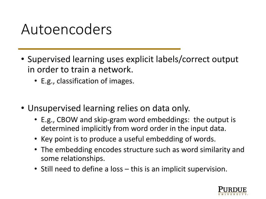


Autoencoders
•
Supervised learning uses explicit labels/correct output
in order to train a network.
•
E.g., classification of images.
•
Unsupervised learning relies on data only.
•
E.g., CBOW and skip-gram word embeddings: the output is
determined implicitly from word order in the input data.
•
Key point is to produce a useful embedding of words.
•
The embedding encodes structure such as word similarity and
some relationships.
•
Still need to define a loss – this is an implicit supervision.

Autoencoders
•
Autoencoders are designed to reproduce their
input, especially for images.
•
Key point is to reproduce the input from a learned
encoding.
https://www.edureka.co/blog/autoencoders-tutorial/
Autoencoders
•
Compare PCA/SVD
•
PCA takes a collection of vectors (images) and produces
a usually smaller set of vectors that can be used to
approximate the input vectors via linear combination.
•
Very efficient for certain applications.
•
Fourier and wavelet compression is similar.
•
Neural network autoencoders
•
Can learn nonlinear dependencies
•
Can use convolutional layers
•
Can use transfer learning
https://www.edureka.co/blog/autoencoders-tutorial/
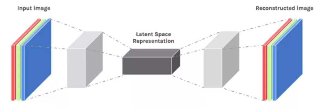
Autoencoders: structure
•
Encoder: compress input into a latent-space of
usually smaller dimension. h = f(x)
•
Decoder: reconstruct input from the latent space.
r = g(f(x)) with r as close to x as possible
https://towardsdatascience.com/deep-inside-autoencoders-7e41f319999f
Autoencoders: applications
•
Denoising: input clean image + noise and train to
reproduce the clean image.
https://www.edureka.co/blog/autoencoders-tutorial/
Autoencoders: Applications
•
Image colorization: input black and white and train
to produce color images
https://www.edureka.co/blog/autoencoders-tutorial/
Autoencoders: Applications
•
Watermark removal
https://www.edureka.co/blog/autoencoders-tutorial/
Properties of Autoencoders
•
Data-specific
: Autoencoders are only able to
compress data similar to what they have been
trained on.
•
Lossy:
The decompressed outputs will be degraded
compared to the original inputs.
•
Learned automatically from examples:
It is easy to
train specialized instances of the algorithm that will
perform well on a specific type of input.
https://www.edureka.co/blog/autoencoders-tutorial/
Capacity
•
As with other NNs, overfitting is a problem when
capacity is too large for the data.
•
Autoencoders address this through some
combination of:
•
Bottleneck layer – fewer degrees of freedom than in
possible outputs.
•
Training to denoise.
•
Sparsity through regularization.
•
Contractive penalty.
Bottleneck layer (undercomplete)
•
Suppose input images are nxn and the latent space
is m < nxn.
•
Then the latent space is not sufficient to reproduce
all images.
•
Needs to learn an encoding that captures the
important features in training data, sufficient for
approximate reconstruction.
Simple bottleneck layer in Keras
•
input_img = Input(shape=(784,))
•
encoding_dim = 32
•
encoded = Dense(encoding_dim, activation='relu')(input_img)
•
decoded = Dense(784, activation='sigmoid')(encoded)
•
autoencoder = Model(input_img, decoded)
•
Maps 28x28 images into a 32 dimensional vector.
•
Can also use more layers and/or convolutions.
https://blog.keras.io/building-autoencoders-in-keras.html
Denoising autoencoders
•
Basic autoencoder trains to minimize the loss
between x and the reconstruction g(f(x)).
•
Denoising autoencoders train to minimize the loss
between x and g(f(x+w)), where w is random noise.
•
Same possible architectures, different training data.
•
Kaggle has a dataset on damaged documents.
https://blog.keras.io/building-autoencoders-in-keras.html
Denoising autoencoders
•
Denoising autoencoders can’t simply memorize the
input output relationship.
•
Intuitively, a denoising autoencoder learns a
projection from a neighborhood of our training
data back onto the training data.
https://ift6266h17.files.wordpress.com/2017/03/14_autoencoders.pdf
Sparse autoencoders
•
Construct a loss function to penalize
activations
within a layer.
•
Usually regularize the
weights
of a network, not the
activations.
•
Individual nodes of a trained model that activate
are
data-dependent.
•
Different inputs will result in activations of different
nodes through the network.
•
Selectively activate regions of the network
depending on the input data.
https://www.jeremyjordan.me/autoencoders/
Sparse autoencoders
•
Construct a loss function to penalize
activations
the
network.
•
L1 Regularization
: Penalize the absolute value of the
vector of activations
a
in layer
h
for observation
I
•
KL divergence:
Use cross-entropy between average
activation and desired activation
https://www.jeremyjordan.me/autoencoders/
Contractive autoencoders
•
Arrange for similar inputs to have similar activations.
•
I.e., the
derivative of the hidden layer activations are
small
with respect to the input.
•
Denoising autoencoders make the
reconstruction function
(encoder+decoder) resist small perturbations of the input
•
Contractive autoencoders make the
feature extraction
function
(ie. encoder) resist infinitesimal perturbations of
the input.
https://www.jeremyjordan.me/autoencoders/
Contractive autoencoders
•
Contractive autoencoders make the
feature
extraction function
(ie. encoder) resist infinitesimal
perturbations of the input.
https://ift6266h17.files.wordpress.com/2017/03/14_autoencoders.pdf
Autoencoders
•
Both the denoising and contractive autoencoder can
perform well
•
Advantage of denoising autoencoder : simpler to implement-
requires adding one or two lines of code to regular
autoencoder-no need to compute Jacobian of hidden layer
•
Advantage of contractive autoencoder : gradient is
deterministic -can use second order optimizers (conjugate
gradient, LBFGS, etc.)-might be more stable than denoising
autoencoder, which uses a sampled gradient
•
To learn more on contractive autoencoders:
•
Contractive Auto-Encoders: Explicit Invariance During Feature
Extraction. Salah Rifai, Pascal Vincent, Xavier Muller, Xavier
Glorot et Yoshua Bengio, 2011.
https://ift6266h17.files.wordpress.com/2017/03/14_autoencoders.pdf
Autoencoders play a crucial role in supervised and unsupervised learning, with applications ranging from image classification to denoising and watermark removal. They compress input data into a latent space and reconstruct it to produce valuable embeddings. Autoencoders are data-specific, lossy, and can be trained automatically for specific input types.

Download Presentation

Please find below an Image/Link to download the presentation.
The content on the website is provided AS IS for your information and personal use only. It may not be sold, licensed, or shared on other websites without obtaining consent from the author.If you encounter any issues during the download, it is possible that the publisher has removed the file from their server.
You are allowed to download the files provided on this website for personal or commercial use, subject to the condition that they are used lawfully. All files are the property of their respective owners.
The content on the website is provided AS IS for your information and personal use only. It may not be sold, licensed, or shared on other websites without obtaining consent from the author.
E N D
Presentation Transcript
Autoencoders Supervised learning uses explicit labels/correct output in order to train a network. E.g., classification of images. Unsupervised learning relies on data only. E.g., CBOW and skip-gram word embeddings: the output is determined implicitly from word order in the input data. Key point is to produce a useful embedding of words. The embedding encodes structure such as word similarity and some relationships. Still need to define a loss this is an implicit supervision.
Autoencoders Autoencoders are designed to reproduce their input, especially for images. Key point is to reproduce the input from a learned encoding. https://www.edureka.co/blog/autoencoders-tutorial/
Autoencoders Compare PCA/SVD PCA takes a collection of vectors (images) and produces a usually smaller set of vectors that can be used to approximate the input vectors via linear combination. Very efficient for certain applications. Fourier and wavelet compression is similar. Neural network autoencoders Can learn nonlinear dependencies Can use convolutional layers Can use transfer learning https://www.edureka.co/blog/autoencoders-tutorial/
Autoencoders: structure Encoder: compress input into a latent-space of usually smaller dimension. h = f(x) Decoder: reconstruct input from the latent space. r = g(f(x)) with r as close to x as possible https://towardsdatascience.com/deep-inside-autoencoders-7e41f319999f
Autoencoders: applications Denoising: input clean image + noise and train to reproduce the clean image. https://www.edureka.co/blog/autoencoders-tutorial/
Autoencoders: Applications Image colorization: input black and white and train to produce color images https://www.edureka.co/blog/autoencoders-tutorial/
Autoencoders: Applications Watermark removal https://www.edureka.co/blog/autoencoders-tutorial/
Properties of Autoencoders Data-specific: Autoencoders are only able to compress data similar to what they have been trained on. Lossy: The decompressed outputs will be degraded compared to the original inputs. Learned automatically from examples: It is easy to train specialized instances of the algorithm that will perform well on a specific type of input. https://www.edureka.co/blog/autoencoders-tutorial/
Capacity As with other NNs, overfitting is a problem when capacity is too large for the data. Autoencoders address this through some combination of: Bottleneck layer fewer degrees of freedom than in possible outputs. Training to denoise. Sparsity through regularization. Contractive penalty.
Bottleneck layer (undercomplete) Suppose input images are nxn and the latent space is m < nxn. Then the latent space is not sufficient to reproduce all images. Needs to learn an encoding that captures the important features in training data, sufficient for approximate reconstruction.
Simple bottleneck layer in Keras input_img = Input(shape=(784,)) encoding_dim = 32 encoded = Dense(encoding_dim, activation='relu')(input_img) decoded = Dense(784, activation='sigmoid')(encoded) autoencoder = Model(input_img, decoded) Maps 28x28 images into a 32 dimensional vector. Can also use more layers and/or convolutions. https://blog.keras.io/building-autoencoders-in-keras.html
Denoising autoencoders Basic autoencoder trains to minimize the loss between x and the reconstruction g(f(x)). Denoising autoencoders train to minimize the loss between x and g(f(x+w)), where w is random noise. Same possible architectures, different training data. Kaggle has a dataset on damaged documents. https://blog.keras.io/building-autoencoders-in-keras.html
Denoising autoencoders Denoising autoencoders can t simply memorize the input output relationship. Intuitively, a denoising autoencoder learns a projection from a neighborhood of our training data back onto the training data. https://ift6266h17.files.wordpress.com/2017/03/14_autoencoders.pdf
Sparse autoencoders Construct a loss function to penalize activations within a layer. Usually regularize the weights of a network, not the activations. Individual nodes of a trained model that activate are data-dependent. Different inputs will result in activations of different nodes through the network. Selectively activate regions of the network depending on the input data. https://www.jeremyjordan.me/autoencoders/
Sparse autoencoders Construct a loss function to penalize activations the network. L1 Regularization: Penalize the absolute value of the vector of activations a in layer h for observation I KL divergence: Use cross-entropy between average activation and desired activation https://www.jeremyjordan.me/autoencoders/
Contractive autoencoders Arrange for similar inputs to have similar activations. I.e., the derivative of the hidden layer activations are small with respect to the input. Denoising autoencoders make the reconstruction function (encoder+decoder) resist small perturbations of the input Contractive autoencoders make the feature extraction function (ie. encoder) resist infinitesimal perturbations of the input. https://www.jeremyjordan.me/autoencoders/
Contractive autoencoders Contractive autoencoders make the feature extraction function (ie. encoder) resist infinitesimal perturbations of the input. https://ift6266h17.files.wordpress.com/2017/03/14_autoencoders.pdf
Autoencoders Both the denoising and contractive autoencoder can perform well Advantage of denoising autoencoder : simpler to implement- requires adding one or two lines of code to regular autoencoder-no need to compute Jacobian of hidden layer Advantage of contractive autoencoder : gradient is deterministic -can use second order optimizers (conjugate gradient, LBFGS, etc.)-might be more stable than denoising autoencoder, which uses a sampled gradient To learn more on contractive autoencoders: Contractive Auto-Encoders: Explicit Invariance During Feature Extraction. Salah Rifai, Pascal Vincent, Xavier Muller, Xavier Glorot et Yoshua Bengio, 2011. https://ift6266h17.files.wordpress.com/2017/03/14_autoencoders.pdf


")