Aerodynamics and Airfoil Dynamics in Incompressible Flow
Exploring the principles of aerodynamics, this content delves into topics such as airfoil nomenclature, vortex sheets, the Kutta condition, Kelvin's circulation theorem, and thin airfoil theory. Detailed explanations and illustrations help in understanding the key concepts related to airflow over airfoils.

Download Presentation

Please find below an Image/Link to download the presentation.
The content on the website is provided AS IS for your information and personal use only. It may not be sold, licensed, or shared on other websites without obtaining consent from the author.If you encounter any issues during the download, it is possible that the publisher has removed the file from their server.
You are allowed to download the files provided on this website for personal or commercial use, subject to the condition that they are used lawfully. All files are the property of their respective owners.
The content on the website is provided AS IS for your information and personal use only. It may not be sold, licensed, or shared on other websites without obtaining consent from the author.
E N D
Presentation Transcript
Chap.4 Incompressible Flow over Airfoils
OUTLINE Airfoil nomenclature and characteristics The vortex sheet The Kutta condition Kelvin s circulation theorem Classical thin airfoil theory The cambered airfoil The vortex panel numerical method
Airfoil nomenclature and characteristics Nomenclature
The vortex sheet Vortex sheet with strength = (s) Velocity at P induced by a small section of vortex sheet of strength ds ds dV 2 = r For velocity potential (to avoid vector addition as for velocity) = 2 ds d
The velocity potential at P due to entire vortex sheet 2 1 b = ds a The circulation around the vortex sheet b ads = The local jump in tangential velocity across the vortex sheet is equal to . = , 2 0 u u dn 1
Calculate (s) such that the induced velocity field when added to V will make the vortex sheet (hence the airfoil surface) a streamline of the flow. The resulting lift is given by Kutta-Joukowski theorem = V L Thin airfoil approximation
The Kutta condition Statement of the Kutta condition The value of around the airfoil is such that the flow leaves the trailing edge smoothly. If the trailing edge angle is finite, then the trailing edge is a stagnation point. If the trailing edge is cusped, then the velocity leaving the top and bottom surface at the trailing edge are finite and equal. Expression in terms of 0 ) TE ( =
Kelvins circulation theorem Statement of Kelvin s circulation theorem The time rate of change of circulation around a closed curve consisting of the same fluid elements is zero.
Classical thin airfoil theory Goal To calculate (s) such that the camber line becomes a streamline. Kutta condition (TE)=0 is satisfied. Calculate around the airfoil. Calculate the lift via the Kutta-Joukowski theorem.
Approach Place the vortex sheet on the chord line, whereas determine = (x) to make camber line be a streamline. Condition for camber line to be a streamline + = ( ) 0 V w s , n where w'(s) is the component of velocity normal to the camber line.
Expression of V,n dz = + 1 sin tan ( ) V V , n dx For small sin tan , dz ( ) ( ) w s w x = ( ) V V , n dx
Expression for w(x) = x w ) ( x ( ( ) d c 2 ) 0 Fundamental equation of thin airfoil theory ) ( 2 x 1 d dz c = ( ) V dx 0
For symmetric airfoil (dz/dx=0) Fundamental equation for ( ) = x 2 1 ( ) d c V 0 Transformation of , x into c c = , ) = 0 1 ( cos 1 ( cos ) x 2 2 Solution ( + sin 1 ( cos ) = ) 2 V
Check on Kutta condition by LHospitals rule sin 2 ) ( = = 0 V cos Total circulation around the airfoil = 0 c = ( ) d cV Lift per unit span L = = 2 V c V
Lift coefficient and lift slope = = c q dc L = 2 , 2 l c l d Moment about leading edge and moment coefficient c q L d M = = 2 c LE 2 0 c M = = = l LE c c , m le 2 2 4 q
Moment coefficient about quarter-chord + = le m c m c c c l , / 4 , 4 = 0 c , / 4 m c For symmetric airfoil, the quarter-chord point is both the center of pressure and the aerodynamic center.
The cambered airfoil Approach Fundamental equation ( 2 1 ) sin d dz = ( ) V cos cos dx 0 0 Solution ( + sin 1 cos = n = + ) 2 sin V A A n 0 n 1 Coefficients A0 and An = 0 A 1 2 dz dz = , cos d A n d 0 0 0 n dx dx 0 0
Aerodynamic coefficients Lift coefficient and slope = 2 c l , 1 dc dz + = (cos ) 1 2 l d 0 0 dx d 0 Form thin airfoil theory, the lift slope is always 2 for any shape airfoil. Thin airfoil theory also provides a means to predict the angle of zero lift. 1 dx dz = ) 1 (cos d = 0 0 0 L 0
Moment coefficients = c + ( ) l c A A , 1 2 m le 4 4 = ( ) c A A , / 4 2 1 m c 4 For cambered airfoil, the quarter-chord point is not the center of pressure, but still is the theoretical location of the aerodynamic center.
The location of the center of pressure + = ( 1 4 c l c ) x A A 1 2 cp Since x as 0 c cp l the center of pressure is not convenient for drawing the force system. Rather, the aerodynamic center is more convenient. The location of aerodynamic center m x ac + = dc dc , / 4 m c 0 where , 25 . 0 , l a m 0 0 a d d 0
The vortex panel numerical method Why to use this method For airfoil thickness larger than 12%, or high angle of attack, results from thin airfoil theory are not good enough to agree with the experimental data. Approach Approximate the airfoil surface by a series of straight panels with strength which is to be determined. j
The velocity potential induced at P due to the j th panel is ds 2 y y 1 j = = 1 j , tan j pj j pj x x j j The total potential at P n n = j = = ( ) P ds j pj j 2 j = 1 1 j j Put P at the control point of i th panel n y x = j = ( , ) ds i i ij j 2 j 1 j
The normal component of the velocity is zero at the control points, i.e. V V n n 0 , = + = n = j ij = where cos i , V V V ds , n n j 2 n j 1 j i n = j ij = = cos , 0 , 1 , V ds i n i j 2 n j 1 j i We then have n linear algebraic equation with n unknowns.
Kutta condition = = ( TE ) 0 1 i i To impose the Kutta condition, we choose to ignore one of the control points. The need to ignore one of the control points introduces some arbitrariness in the numerical solution.


 such that the induced velocity field")


")
")