Algorithm Strategies: Greedy Algorithms and the Coin-changing Problem
This topic delves into general algorithm strategies, focusing on the concept of greedy algorithms where locally optimal choices are made with the hope of finding a globally optimal solution. The discussion includes the nature of greedy algorithms, examples such as Dijkstra's algorithm and Prim's algorithm, as well as an illustration of the coin-changing problem. While greedy algorithms may not always lead to the optimal solution, they can provide good approximate solutions in certain scenarios.
Download Presentation

Please find below an Image/Link to download the presentation.
The content on the website is provided AS IS for your information and personal use only. It may not be sold, licensed, or shared on other websites without obtaining consent from the author. Download presentation by click this link. If you encounter any issues during the download, it is possible that the publisher has removed the file from their server.
E N D
Presentation Transcript
ECE365: Data Structures and Algorithms II (DSA 2) Algorithm Strategies
Algorithm Strategies In our two DSA courses, we have discussed algorithms to solve various problems and analyzed their running times We have not yet discussed how to solve problems ourselves (i.e., how to design algorithms to compute solutions to problems) To a large extent, this generally involves some creativity Also keep in mind that some problems that sound simple may not have any efficient solutions (or may not have solutions at all) In this topic, we will discuss some general algorithm strategies that may help you to determine methods for solving a given problem We will also discuss at least one new example of each type of algorithm This topic has been largely based on Chapter 10 of the textbook, titled "Algorithm Design Techniques" We will cover some of the subtopics in more detail than the textbook
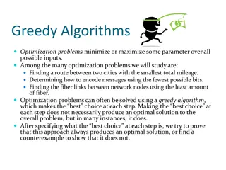
Greedy Algorithms The idea behind a greedy algorithm is to make a sequence of choices such that each choice seems to be the best choice possible at the time that you make it In general, you are making locally optimal choices, perhaps with the hope of finding a globally optimal solution Sometimes, you can then prove that the final solution will be the best solution possible; other times, this will not be the case at all If you need an algorithm that is guaranteed to find an optimal solution, then you need to prove that the algorithm is optimal; in some cases, an inductive proof can be used Even when greedy algorithms do not find the optimal solution (e.g., for the traveling salesman problem), they might be guaranteed or likely to find a good solution close to the optimal solution When you use such a greedy algorithm, you are using it as a heuristic We have already seen examples of greedy algorithms when discussing graph algorithms These include Dijkstra's algorithm to solve the single-source shortest-path problem and Prim's algorithm for determining a minimum spanning tree
The Coin-changing Problem We will start with a simple example of a greedy algorithm that we might apply to the coin-changing problem The problem asks you to make change for a specified amount of money using the smallest number of coins possible Some versions of the problem accept the values of available coins as part of the input For example, if an amount is specified, and we are using U.S. currency, you can use as many quarters as possible, then dimes, then nickels, and then pennies We will not prove it, but this greedy algorithm will lead to the best possible solution when applied to U.S. currency However, if the types of coins available are 11-cent coins, 5-cent coins, and 1-cent coins, this solution would not lead to an optimal solution To see this, consider making change for 15 cents
Simple Scheduling Problem A simple example of a scheduling problem involves a set of jobs, j1, j2, jN, all with known running times t1, t2, , tN To start, assume that there is a single processor available We are assuming non-preemptive scheduling, meaning that once a job stars, it must run until completion We want to schedule the jobs in order to achieve the minimum average completion time A solution that is optimal is to sort the jobs in terms of their running time (from shortest to longest) and schedule them in that order Even if there are multiple processors, you can cycle through the processors, assigning jobs in sorted order This is also guaranteed to be optimal (we won t prove it), although this is not necessarily the only optimal solution However, a similar-sounding problem that asks you to minimize the final completion time when multiple processors are involved is NP-complete!
Huffman Codes The next greedy algorithm we will discuss is a very popular compression algorithm involving Huffman code The algorithm is known as Huffman coding or Huffman encoding Consider a file that contains C distinct types of characters Then a system that uses the same number of bits per character requires at least logC bits per character ASCII uses 8 bits per character, although only 7 would really be necessary for standard ASCII Standard ASCII encodes 128 distinct characters, of which approximately 100 are printable According to our textbook, Huffman codes typically save about 25% of space for typically large files, and up to 50% or 60% on many large data files According to another source (by Cormen, Leiserson, Rivest, and Stein), anywhere from 20% to 90% savings is typical
Huffman Coding Example We will examine an example from the book that assumes the existence of only 7 distinct characters Specifically, the distinct characters are: 'a', 'e', 'i', 's', 't', space, and newline If the same number of bits were used for each character, 3 bits per character would be required We will assume that the frequency of each character in the file has already been computed In our example, we will posit that there are 10 a s 15 e s, 12 i s, 3 s s, 4 t s, 13 spaces, and 1 newline The figure on the next slide shows that for this case, a standard encoding would require 174 bits
Tries We can represent such encodings with a special type of binary tree known as a trie In a trie, left branches represent the bit 0, right branches represent the bit 1, and characters are indicated by the leaves Some sources allow the branches of a trie to represent more general characters, or allow internal nodes to represent characters, but that will not be necessary for Huffman coding The standard encoding we have seen can be represented by the following trie:
Slightly Better Trie This is clearly not the most efficient encoding Note that the only character with a code that starts with 11 is the newline, so the following zero does not provide any useful information An optimal trie for encoding will always be a full binary tree (i.e., all nodes will either be leaves or have two children) A slightly better, but still far-from-optimal, trie is as follows:
Prefix codes Any encoding in which no character code is a prefix of another character code is known as a prefix code Prefix codes also include that files encoded using them will be unambiguous When a file has been encoded using a prefix code, we can easily decode it even though character codes may have a different lengths Forcing a trie to indicate each distinct character as a leaf ensures that the trie represents a prefix code The goal of Huffman coding is to find the optimal trie, i.e., the optimal prefix code The principal behind this is to use shorter codes for frequent characters and longer codes for rare characters The optimal trie for the example we have been dealing with is shown on the next slide The slide after that shows that this encoding would require 146 bits to encode the file
Analyzing the Optimal Trie and Prefix Code There are many prefix codes that tie for optimal For example, swapping leaves at the same level of the trie or swapping left and right links of internal nodes lead to equally efficient encodings In general, if each character cioccurs fitimes and is at depth diin the trie, then the cost of the using code to encode the file is equal to idi* fi For this example, a standard encoding uses 174 bits, while the optimal encoding uses 146 bits This is only a savings of 16.1%, but that is because we were only dealing with a small file that contains only 7 distinct characters The normal ASCII character set has about 100 printable characters, but many occur very rarely, and some occur much more frequently than others
Huffmans Algorithm A greedy algorithm for finding an optimal trie was created by David Huffman in 1952 while he was a graduate student at M.I.T. Let's say that the number of distinct characters in a text file to be compressed is C Huffman's algorithm maintains a forest of tries; the weight of each trie is equal to the sum of the frequencies of its leaves At the start, there are C single-node tries representing each of the characters Through each of C-1 iterations, the two tries, T1 and T2, of smallest weight are selected (breaking ties arbitrarily) A new trie is formed with a new root and T1 and T2 as subtrees At the end of the algorithm, there is one trie remaining, and this is an optimal trie representing an optimal prefix encoding This algorithm can be implemented efficiently using a priority queue (e.g., a binary heap) The next slide shows my pseudo-code for the algorithm
Huffman Algorithm Pseudo-code Huffman ( Set-of-characters C ) initialize Q as empty priority queue for each character c in C create a single-node trie T T.data c T.frequency c.frequency Insert(Q, T) loop |C| - 1 times T1 DeleteMin(Q) T2 DeleteMin(Q) create a new trie T T.left T1 T.right T2 T.frequency T1.frequency + T2.frequency Insert(Q, T) return DeleteMin(Q)
Analyzing the Huffman Algorithm If C is the number of distinct characters, there will be C-1 iterations Each iteration require O(log C) time (using binary heaps), so the running time of this algorithm is O(C log C) This assumes that the frequency of each character is known Otherwise, an additional loop is necessary at the start of the routine that takes linear time with respect to the size of the file Although this does not change the complexity, this linear loop will probably take longer than the rest of the algorithm This is because C is generally going to be small, and we probably won t bother compressing a file if it isn t large Even if we use a simpler, quadratic implementation, O(C2), for the main Huffman routine, it will be fast
Why Does This Work? We will informally discuss why this algorithm is guaranteed to produce the optimal solution Recall that the optimal trie must be a full trie Therefore, the deepest leaf must have a sibling (another leaf); clearly, these nodes should represent the two least frequent characters The first pass of the algorithm therefore produces a valid part of the trie You can then consider the merged tree to represent a meta-character with a frequency equal to the sum of the characters represented by its leaves Therefore, the later iterations of the algorithm are correct for the same reason as the first; it is always valid to combine the two least-frequent metacharacters Whenever we merge two trees, we are adding a bit to the representation of each leaf of both trees Each greedy step adds the least number of bits possible to the final trie
Using Huffman Codes Once the trie representing the optimal encoding is produced, it can be used to compress the file A representation of the encoding must be included with the compressed file (either internal to the file or along with it) Otherwise, the decoding of the file will not be possible This representation could take the form of a chart that maps binary sequences to characters Alternatively, it could take the form of a data structure representing the trie In some other contexts, the prefix code is determined based on a large dataset once, and then applied to future files This is not optimal for each individual file, but it allows a single shared compression scheme to be applied to many files
Divide and Conquer Algorithms The next strategy we will discuss is called divide-and-conquer This strategy is applicable when a problem can be broken down into parts that can be solved with a similar algorithm to the original problem There must be some way to combine the solutions to the parts to form a final solution The parts (smaller problems) are often solved with recursion (although recursion is never necessary to implement a solution) There also must be a base case for which a recursive call does not apply We have already seen examples of divide-and-conquer algorithms when discussing sorting in Data Structures and Algorithms I These include mergesort, quicksort, and quickselect We have seen that the Master theorem can sometimes be used to determine the running time complexity of such an algorithm
Examples Discussed in Textbook The textbook discusses the following divide-and-conquer algorithms: An algorithm for finding the closest pair of points out of a set of N points in O(N log N) time A worst-case linear algorithm for selection involving median-of-median-of- five pivot selection for quickselect An algorithm for multiplying two N-digit numbers in O(N1.59) time An algorithm for matrix multiplication that runs in O(N2.81) time We will go over a different problem that I consider fun, although not of practical significance (and the solution is exponential)
Tower of Hanoi The Tower of Hanoi is a puzzle including three sticks and disks that can be placed on them At the start, all disks are on one of the stick, arrange from largest (at the bottom) to the smallest (at the top) The goal is to move the disks from the starting stick to a designated destination stick, subject to the following rules: Only one disk can be moved at a time You can only lift the top disk off a stick; this disk may then be placed on another stick, as long as it does not violate the next constraint You can never place a larger disk on top of a smaller disk
Solving the Tower of Hanoi Assume we have a Tower of Hanoi puzzle with N disks At some point, we need to move the largest disk from the source stick to the destination stick Before that, we must move the other N-1 disks from the source stick to the auxiliary stick The largest disk will not affect any of the moves required to achieve that intermediate goal After the largest disk is moved to the destination stick, when then must move the other N-1 disks from the auxiliary stick to the destination stick In summary, we can move N disks from the source stick to the destination stick with the following steps: 1. Move N-1 disks from the source stick to the auxiliary stick (this is a recursive step) 2. Move the largest disk from the source stick to the destination stick 3. Move N-1 disks from the auxiliary stick to the destination stick (this is a recursive step) Note that all three of the steps listed in this solution are necessary
Code for Solving the Tower of Hanoi void Tower(int n, string src, string dst, string aux) { if (n == 1) cout << "Move from " << src << " to " << dst << "\n"; else { Tower(n-1, src, aux, dst); cout << "Move from " << src << " to " << dst << "\n"; Tower(n-1, aux, dst, src); } return; } Suppose the disks are labeled "A", "B", and "C", and there are 8 disks that must be moved from "A" to "C"; then we could call the above function as follows: Tower(8, "A", "C", "B");
Analyzing the Solution Suppose T(N) is the number of moves used to solve the puzzle with our solution when there are N disks The equation describing the number of steps used to solve the problem can be described by the following recurrence relation: T(N) = 2 * T(N - 1) + O(1) On the surface, this might look similar to the mergesort recurrence However, note that each recursive call here is applied to N-1, not to N/2 This makes a huge difference; unlike other divide-and-conquer solutions we have seen, this is an exponential solution We could clearly see that, as each value of T(N) more than doubles as N increases by 1 This does not mean it is a bad solution, as far as solutions to this problem go An exponential number of moves are required to solve this problem, and it can be shown that this solution uses the fewest moves possible
Dynamic Programming Algorithms The next strategy we will discuss is known as dynamic programming Dynamic programming is related to divide-and-conquer and recursive algorithms When dealing with straight-forward implementations of recursive algorithms, algorithms can become much less efficient than necessary if the subproblems are not independent We ll start by discussing implementations for computing the kthvalue in the Fibonacci sequence (1, 1, 2, 3, 5, 8, 13, 21, 34, 55, etc.), which we discussed early in DSA 1 Really, we are computing the right-most 32-bits of values, since we are not worrying about overflow We learned that a typical recursive solution is an exponential time solution We also saw that a standard iterative solution is linear, and it only needs to keep track of the two previous values in the Fibonacci sequence (and the current value) However, consider a more general recursive mathematical function for which the current value depends not only on the previous two values, but perhaps on all previous values This can still be solved iteratively by storing all the values computed so far in an array We can also take this approach for Fibonacci, even though it uses more memory than necessary
Fibonacci Implementations (from DSA1) Recursive Solution (exponential!) int Fibonacci(int n) { if (n <= 2) return 1; else return (Fibonacci(n-1) + Fibonacci(n-2)); } Iterative Solution (linear) int Fibonacci(int n) { int prev1 = 1, prev2 = 1; int x, cur; if (n <= 2) return 1; else { for (x = 3; x <= n; x++, prev2 = prev1, prev1 = cur) cur = prev2 + prev1; return cur; } }
Recursive Fibonacci is Exponential One way to show that the recursive implementation is an exponential time solution is to examine a tree representing the recursive calls; for example: Another way involves analyzing the number of computational steps the routine requires and comparing this to the formula defining the Fibonacci sequence: T(N) = T(N - 1) + T(N - 2) + c Fib(N) = Fib(N - 1) + Fib(N - 2) Conclusion: The simplest or most obvious way to compute something is not always the most efficient!
Bottom-Up Dynamic Programming To the right, we see pseudo-code for an iterative Fibonacci implementation This version uses linear memory, which is more than necessary However, there are a couple of advantages: This version is more readable than the previous version This version is easily expandable to functions that rely on many previous values This is an example of bottom-up dynamic programming, meaning that: We are storing the computed values in an array (or more general matrix) Each newly computed value depends on other values that have already been computed Fibonacci( integer N ) if N 2 return 1 Fib[1] 1 Fib[2] 1 Loop i from 3 to N Fib[i] Fib[i-1] + Fib[i-2] return Fib[n]
Top-Down Dynamic Programming To the right, we see pseudo-code for a recursive Fibonacci implementation Although recursive, this function executes in linear time, just like the iterative solution Any call asking for a value that has already been computed will execute in quick constant time The array "known" could be a global array, a static variable, or a parameter passed by reference The array must be large enough to hold N values, all initialized to all "unknown" This is an example of top-down dynamic programming, meaning that: We store the computed values in an array (or more general matrix) after they are computed via recursive calls The start of each recursive routine checks to see if the desired value has already been computed If so, it just looks retrieves and returns the value The use of the array or matrix is called memoization Fibonacci( integer N ) if known[N] != unknown return known[N] if N 2 v 1 else v Fibonacci(N-1)+Fibonacci(N-2) known[N] v return v
The Longest Common Subsequence Problem We will use dynamic program to solve the Longest Common Subsequence Problem (LCSP); note that this problem is not discussed in the textbook This involves a different definition of a subsequence than the Maximum Subsequence Sum Problem that we discussed near the start of Data Structures and Algorithms I Consider a string: X = x1x2x3...xn A subsequence of X is any string Z = z1z2z3...zkfor which there exists a strictly increasing sequence i1, i2, ..., ik such that for all j=1, 2, ..., k, it is true that zj= xij Now consider two strings: X as defined above and also Y = y1y2y3...ym The Longest Common Subsequence Problem asks us to determine the longest string, Z, that is a subsequence of both X and Y One possible way to do this would be to exhaustively examine every subsequence of X and check if it is also a subsequence of Y However, there are 2npossible subsequences of X, and checking if each is a subsequence of Y would take time linear to m, so this would be an (2n* m) solution Instead, we are going to use an efficient dynamic programming solution
Solving the LCSP To solve the problem, we are going to use a matrix M with n+1 rows (numbered 0 through n) and m+1 columns (numbered 0 through m) M[i, j] represents the length of the longest common subsequence of the strings x1x2x3...xiand y1y2y3...yj We start by filling in the first column and first row with zeros; this is because the length of the longest common subsequence is 0 if one of the two strings is empty We are going to fill in the rest of the matrix one row at a time, from top to bottom, filling each row from left to right Let's say we want to fill in a particular slot M[i, j] and we have already filled in all the slots above this slot and all the slots to the left of this slot in the current row We can then say that if xi== yj, M[i, j] must equal M[i-1, j-1] +1 Otherwise, M[i, j] will be the maximum of M[i-1, j] and M[i, j-1] At the end of the algorithm, the length of the longest common subsequence is stored at the bottom right of the matrix, in M[n, m] Note that this is clearly a O(n * m) time algorithm This is a bottom-up approach; a top-down approach is also possible
LCSP Pseudo-code LongestCommonSubsequence ( String X, String Y ) n length(X) m length(Y) loop i from 0 to m M[0,i] 0 Loop i from 0 to n M[i,0] 0 Loop i from 1 to n Loop j from 1 to m if Xi== Yj M[i, j] M[i-1, j-1] + 1 else if M[i-1, j] M[i, j-1] M[i, j] M[i-1, j] else M[i, j] M[i, j-1]
LCSP Example Consider finding the longest common subsequence of X = "wired" and Y = "world" The matrix would then be 6 x 6, initialized as follows: w o r l d 0 1 2 3 4 5 0 0 0 0 0 0 0 w 1 0 i 2 0 r 3 0 e 4 0 d 5 0
LCSP Example (continued) We not loop through the rows one at a time from left to right one at a time, starting at position (1, 1) Since the two w s match, this entry becomes M[0, 0] + 1 = 1 w o r l d 0 1 2 3 4 5 0 0 0 0 0 0 0 w 1 0 1 i 2 0 r 3 0 e 4 0 d 5 0
LCSP Example (continued) Next, we fill in position (1, 2) The w and o do not match, so this is max(M[0, 2], M[1, 1]) = 1 w o r l d 0 1 2 3 4 5 0 0 0 0 0 0 0 w 1 0 1 1 i 2 0 r 3 0 e 4 0 d 5 0
LCSP Example (continued) We continue filling in row 1 w o r l d 0 1 2 3 4 5 0 0 0 0 0 0 0 w 1 0 1 1 1 i 2 0 r 3 0 e 4 0 d 5 0
LCSP Example (continued) We continue filling in row 1 w o r l d 0 1 2 3 4 5 0 0 0 0 0 0 0 w 1 0 1 1 1 1 i 2 0 r 3 0 e 4 0 d 5 0
LCSP Example (continued) We continue filling in row 1 w o r l d 0 1 2 3 4 5 0 0 0 0 0 0 0 w 1 0 1 1 1 1 1 i 2 0 r 3 0 e 4 0 d 5 0
LCSP Example (continued) Now, we start the next row at position (2, 1) Since the i and w do not match, we again take the maximum of the value to the left and the value above w o r l d 0 1 2 3 4 5 0 0 0 0 0 0 0 w 1 0 1 1 1 1 1 i 2 0 1 r 3 0 e 4 0 d 5 0
LCSP Example (continued) We continue filling in the row 2 w o r l d 0 1 2 3 4 5 0 0 0 0 0 0 0 w 1 0 1 1 1 1 1 i 2 0 1 1 r 3 0 e 4 0 d 5 0
LCSP Example (continued) We continue filling in the row 2 w o r l d 0 1 2 3 4 5 0 0 0 0 0 0 0 w 1 0 1 1 1 1 1 i 2 0 1 1 1 r 3 0 e 4 0 d 5 0
LCSP Example (continued) We continue filling in the row 2 w o r l d 0 1 2 3 4 5 0 0 0 0 0 0 0 w 1 0 1 1 1 1 1 i 2 0 1 1 1 1 r 3 0 e 4 0 d 5 0
LCSP Example (continued) We continue filling in the row 2 w o r l d 0 1 2 3 4 5 0 0 0 0 0 0 0 w 1 0 1 1 1 1 1 i 2 0 1 1 1 1 1 r 3 0 e 4 0 d 5 0
LCSP Example (continued) Now we start filling in row 3 in a similar fashion w o r l d 0 1 2 3 4 5 0 0 0 0 0 0 0 w 1 0 1 1 1 1 1 i 2 0 1 1 1 1 1 r 3 0 1 e 4 0 d 5 0
LCSP Example (continued) Now we start filling in row 3 in a similar fashion w o r l d 0 1 2 3 4 5 0 0 0 0 0 0 0 w 1 0 1 1 1 1 1 i 2 0 1 1 1 1 1 r 3 0 1 1 e 4 0 d 5 0
LCSP Example (continued) When we get to cell (3, 3), the r s match, so this cell takes the value of M[2, 2] + 1 = 2 w o r l d 0 1 2 3 4 5 0 0 0 0 0 0 0 w 1 0 1 1 1 1 1 i 2 0 1 1 1 1 1 r 3 0 1 1 2 e 4 0 d 5 0
