Insights into Genome Assembly and Shotgun Sequencing
Explore the world of genome assembly, shotgun sequencing, and the fundamental concepts behind deriving genomes from large sets of sequencing reads. Learn about the complexity and core algorithms involved in contemporary genome assembly processes. Discover how the shotgun concept has revolutionized genomics and enabled researchers to unravel the mysteries hidden within the genetic code.

Download Presentation

Please find below an Image/Link to download the presentation.
The content on the website is provided AS IS for your information and personal use only. It may not be sold, licensed, or shared on other websites without obtaining consent from the author. Download presentation by click this link. If you encounter any issues during the download, it is possible that the publisher has removed the file from their server.
E N D
Presentation Transcript
Assembling Genomes BCH394P/364C Systems Biology / Bioinformatics Edward Marcotte, Univ of Texas at Austin
www.yourgenome.org/facts/timeline-the-human-genome-project Nature 409, 860-921(2001)
Beijing Genomics Institute If it tastes good you should sequence it... you should know what's in the genes of that species Wang Jun, Chief executive, BGI (Wikipedia)
The NovaSeq in the UT GSAF core generates >1.4 terabases of sequence in a 1-day run Illumina Many millions of 75-150 bp reads
mapping shotgun sequencing
Contemporary genome assembly is fairly complex, but at its core are assembly algorithms that grew from the shotgun concept Twelve quick steps for genome assembly and annotation in the classroom PLoS Comp Biology (2020), doi:10.1371/journal.pcbi.1008325
Beverly Micro Pure White Hell Jigsaw Puzzle (10,000,000,000 Piece)
Thinking about the basic shotgun concept Start with a very large set of random sequencing reads How might we match up the overlapping sequences? How can we assemble the overlapping reads together in order to derive the genome?
Thinking about the basic shotgun concept At a high level, the first genomes were sequenced by comparing pairs of reads to find overlapping reads Then, building a graph (i.e., a network) to represent those relationships The genome sequence is a walk across that graph
The Overlap-Layout-Consensus method Overlap: Compare all pairs of reads (allow some low level of mismatches) Layout: Construct a graph describing the overlaps sequence overlap read read Simplify the graph Find the simplest path through the graph Consensus: Reconcile errors among reads along that path to find the consensus sequence
Building an overlap graph 3 5 EUGENE W. MYERS. Journal of Computational Biology. Summer 1995, 2(2): 275-290
Building an overlap graph Reads 3 5 Overlap graph EUGENE W. MYERS. Journal of Computational Biology. Summer 1995, 2(2): 275-290 (more or less)
Simplifying an overlap graph 1. Remove all contained nodes & edges going to them EUGENE W. MYERS. Journal of Computational Biology. Summer 1995, 2(2): 275-290 (more or less)
Simplifying an overlap graph 2. Transitive edge removal: Given A B D and A D , remove A D EUGENE W. MYERS. Journal of Computational Biology. Summer 1995, 2(2): 275-290 (more or less)
Simplifying an overlap graph 3. If un-branched, calculate consensus sequence If branched, assemble un-branched bits and then decide how they fit together EUGENE W. MYERS. Journal of Computational Biology. Summer 1995, 2(2): 275-290 (more or less)
Simplifying an overlap graph contig (assembled contiguous sequence) EUGENE W. MYERS. Journal of Computational Biology. Summer 1995, 2(2): 275-290 (more or less)
This basic strategy was used for most of the early genomes. Also useful: mate pairs 2 reads separated by a known distance Read #1 DNA fragment of known size Read #2 Contigs can be ordered using these paired reads Contig #1 Contig #2 to produce scaffolds
GigAssembler (used to assemble the public human genome project sequence) Jim Kent David Haussler Let s take a little walk through history to see what they did
Whole genome Assembly: big picture http://www.nature.com/scitable/content/anatomy-of-whole-genome-assembly-20429
GigAssembler Preprocessing 1. Decontaminating & Repeat Masking. 2. Aligning of mRNAs, ESTs, BAC ends & paired reads against initial sequence contigs. psLayout BLAT 3. Creating an input directory (folder) structure.
GigAssembler: Build merged sequence contigs ( rafts )
Sequencing quality (Phred Score) Base-calling Error Probability http://en.wikipedia.org/wiki/Phred_quality_score
Were going to skip the remaining details of GigAssembler (mainly of historical interest now) to get to the key strategy for assembling all of the various contigs and paired end reads into a genome
GigAssembler: Build a raft-ordering graph
GigAssembler: Build a raft-ordering graph Add information from mRNAs, ESTs, paired plasmid reads, BAC end pairs: building a bridge Different weight to different data type: (mRNA ~ highest) Conflicts with the graph as constructed so far are rejected. Build a sequence path through each raft. Fill the gap with N s. 100: between rafts 50,000: between bridged barges
Finding the shortest path across the ordering graph using the Bellman-Ford algorithm http://compprog.wordpress.com/2007/11/29/one-source-shortest-path-the-bellman-ford-algorithm/
Find the shortest path to all nodes. Take every edge and try to relax it (N 1 times where N is the count of nodes) +5 B C -2 +6 +8 -3 A +7 -4 +7 D E +2 +9
Find the shortest path to all nodes. Take every edge and try to relax it (N 1 times where N is the count of nodes) +5 B C -2 +6 +8 -3 A +7 -4 +7 D E +2 +9
Find the shortest path to all nodes. Take every edge and try to relax it (N 1 times where N is the count of nodes) +5 B C Inf. Inf. -2 +6 +8 -3 A +7 START -4 +7 D E +2 Inf. Inf. +9
Find the shortest path to all nodes. Take every edge and try to relax it (N 1 times where N is the count of nodes) +5 B +6 ( A) C Inf. -2 +6 +8 -3 A 0 +7 START -4 +7 D +7 E +2 Inf. +9 ( A)
Find the shortest path to all nodes. Take every edge and try to relax it (N 1 times where N is the count of nodes) +5 B +6 ( A) C +4 ( D) -2 +6 +8 -3 A 0 +7 START -4 +7 D +7 E +2 +2 +9 ( A) ( B)
Find the shortest path to all nodes. Take every edge and try to relax it (N 1 times where N is the count of nodes) +5 B +2 ( C) C +4 ( D) -2 +6 +8 -3 A 0 +7 START -4 +7 D +7 E +2 +2 +9 ( A) ( B)
Find the shortest path to all nodes. Take every edge and try to relax it (N 1 times where N is the count of nodes) +5 B +2 ( C) C +4 ( D) -2 +6 +8 -3 A 0 +7 START -4 +7 D +7 E -2 ( B) +2 +9 ( A)
Answer: A-D-C-B-E +5 B +2 ( C) C +4 ( D) -2 +6 +8 -3 A 0 +7 START -4 +7 D +7 E -2 ( B) +2 +9 ( A)
Modern assemblers now work a bit differently, using so-called DeBruijn graphs: Here s what we saw before: In Overlap-Layout-Consensus: Nodes are reads Edges are overlaps Nature Biotech 29(11):987-991 (2011)
Modern assemblers now work a bit differently, using so-called DeBruijn graphs: In a DeBruijn graph: Nature Biotech 29(11):987-991 (2011)
Why Eulerian? From Leonhard Euler s solution in 1735 to the Bridges of K nigsberg problem: K nigsberg (now Kaliningrad, Russia) had 7 bridges connecting 4 parts of the city. Could you visit each part of the city, walking across each bridge only once, & finish back where you started? Euler conceptualized it as a graph: Nodes = parts of city Edges = bridges (Visiting every edge once = an Eulerian path) Nature Biotech 29(11):987-991 (2011)
DeBruijn graph assemblers tend to have nice properties, e.g. correcting sequencing errors & handling repeats better Sequencing errors appear as bulges Removing the bulges corrects the errors (e.g. leaves the red path) Nature Biotech 29(11):987-991 (2011)
e.g. Velvet, an example algorithm using DeBruijn graphs Beginner s guide to comparative bacterial genome analysis using next-generation sequence data Microb Informatics Exp (2013) doi:10.1186/2042-5783-3-2
Once a reference genome is assembled, new sequencing data can simply be mapped to the reference. reads Reference genome
Mapping reads to assembled genomes The list is a little longer now! e.g. see https://en.wikipedia.org/wiki/ List_of_sequence_alignment_software#Short-Read_Sequence_Alignment Trapnell C, Salzberg SL, Nat. Biotech., 2009
Mapping strategies Trapnell C, Salzberg SL, Nat. Biotech., 2009
Burroughs Wheeler indexing Trapnell C, Salzberg SL, Nat. Biotech., 2009
Burroughs-Wheeler transform indexing BWT is often used for file compression (like bzip2), here used to make a fast lookup index in a genome BWT = reversible block-sorting Input SIX.MIXED.PIXIES.SIFT.SIXTY.PIXIE.DUST.BOXES This sequence is more compressible Forward BWT Output TEXYDST.E.IXIXIXXSSMPPS.B..E.S.EUSFXDIIOIIIT Reverse BWT Recovered input SIX.MIXED.PIXIES.SIFT.SIXTY.PIXIE.DUST.BOXES http://en.wikipedia.org/wiki/Burrows-Wheeler_transform
Burroughs-Wheeler transform indexing http://en.wikipedia.org/wiki/Burrows-Wheeler_transform
Burroughs-Wheeler transform indexing http://en.wikipedia.org/wiki/Burrows-Wheeler_transform


")


")
")