Distributed Biconnectivity in Graph Analysis for Efficient Network Solutions

Graph biconnectivity is a crucial concept in network analysis, ensuring connectivity even when vertices are removed. Efficient distributed biconnectivity algorithms have practical applications in identifying single points of failure in networks. Leveraging previous work on Ice Sheet Connectivity, a new distributed biconnectivity algorithm, BCC-ICE, is proposed to find biconnected components in general graphs.

Download Presentation

Please find below an Image/Link to download the presentation.
The content on the website is provided AS IS for your information and personal use only. It may not be sold, licensed, or shared on other websites without obtaining consent from the author. Download presentation by click this link. If you encounter any issues during the download, it is possible that the publisher has removed the file from their server.
E N D
Presentation Transcript
Distributed Biconnectivity Ian Bogle12George Slota1Sivasankaran Rajamanickam2Karen Devine2 1Rensselaer Polytechnic Institute Troy, NY 2Sandia National Laboratories Albuquerque, NM 1
Graph Biconnectivity is a stronger version of graph connectivity Biconnected Components of a graph remain connected if any single vertex is removed. Articulation Points (or Cut Vertices) are vertices that disconnect the graph if removed. Graph Biconnectivity finds all biconnected components in an input graph 2
Efficient Distributed Biconnectivity algorithms have practical applications Biconnectivity algorithms are useful for finding single points of failure in power and communications networks, as well as processing social networks Finding articulation points in meshes can help solvers converge We are not aware of any distributed parallel biconnectivity algorithms Efficient shared memory biconnectivity algorithms may not lend themselves to an efficient distributed memory implementation A new approach could lead to a more efficient distributed biconnectivity algorithm 3
Our previous work implemented a distributed algorithm that solved a similar problem Determined whether certain parts of an Ice Sheet mesh were adequately connected During this work we realized we could use this Ice Sheet Connectivity algorithm (ICE-CONN) to find biconnected components in a general graph The distributed biconnectivity algorithm (BCC-ICE) we propose leverages the ICE-CONN algorithm 4
Degenerate Features are Parts of the Mesh That Can Rotate or Translate Icebergs Floating Peninsulas (Floating Hinges) Any part of the mesh that can freely rotate or translate makes the velocity solution not unique Blue ice is floating Brown ice is on the ground
Previous Work: Efficiently Detect Degenerate Mesh Features Ice sheet simulations fail to converge due to features like hinged peninsulas and icebergs in meshes New algorithm that detects all degenerate features Distributed memory implementation provides good strong scaling and weak scaling up to 4096 processors Detection takes at most 0.4% of a simulation step s runtime 46,000x faster than previously used preprocessing on highest resolution meshes This work won a Best Paper award, published in Bogle, Devine, Perego, Rajamanickam, and Slota. A Parallel Graph Algorithm for Detecting Mesh Singularities in Distributed Memory Ice Sheet Simulations. Proceedings of the 48th International Conference on Parallel Processing. 2019. 6
Application Provides a Mesh and Grounding Information Legend Floating Touching Ground 7
Degenerate Mesh Features Have at Most One Connection to the Ground These two vertices allow for two unique connections to ground. Only one unique connection to ground exists, it is through this vertex. There are no Degenerate Features These are Degenerate Features Vertex that is floating in the water Vertex that is touching the ground 8
We Identify Parts of the Mesh with No Degenerate Features Legend Degenerate Not Degenerate 9
The ICE-CONN Algorithm Propagates Grounding Information Through the Mesh The ICE-CONN algorithm has two steps: Find Potential Articulation Points Propagate Grounding Information We exploit mesh boundary information to identify potential articulation points Propagating grounding information reveals degenerate mesh features Note: Examples show quad meshes, but the approach works with triangular meshes as well. 10
Step 1: Find Potential Articulation Points Application identifies boundary edges at interfaces between ice and water 11
Step 1: Find Potential Articulation Points This is the only actual Articulation Point Vertices with more than two incident red edges are Potential Articulation Points 12
Step 2: Propagate Grounding Information Legend Start with grounding given from the application Floating Initially Grounded 1 Path to Ground 2 Paths to Ground Potential Articulation Point P P P P 13
Step 2: Propagate Grounding Information Legend Initially grounded vertices have one path to ground Floating Initially Grounded 1 Path to Ground 2 Paths to Ground Potential Articulation Point P P P P 14
Step 2: Propagate Grounding Information Legend Propagate only from vertices that have changed color Floating Initially Grounded 1 Path to Ground 2 Paths to Ground Potential Articulation Point P P P P 15
Step 2: Propagate Grounding Information Legend Stop the propagation at the Potential Articulation Points Floating Initially Grounded 1 Path to Ground 2 Paths to Ground Potential Articulation Point P P P P 16
Step 2: Propagate Grounding Information Legend Floating Initially Grounded 1 Path to Ground 2 Paths to Ground Potential Articulation Point P P P P These two Potential Articulation Points allow for two paths to ground 17
Final Result of the ICE-CONN Algorithm Legend Keep all vertices with two unique paths to the ground Floating Initially Grounded 1 Path to Ground 2 Paths to Ground Potential Articulation Point P P P P These green vertices have two unique paths through both Potential Articulation Points The yellow vertices only have one unique path through this vertex 18
The ICE-CONN Algorithm scales well for mesh inputs 13 Million vertices Strong scaling # Vertices Our Algorithm (Ranks) Matlab Preprocessing 52,465 0.0176 s (6) 1.04 s 210,170 0.0217 s (24) 5.65 s 841,346 0.0414 s (96) 34.60 s 3,368,275 0.0407 s (384) 245.00 s Weak scaling 52k Vertices/Rank 13,479,076 0.0561 s (1536) 2630.00 s Comparison against Matlab preprocessing in Tuminaro, Perego, Tezaur, Salinger, Price. A matrix dependent/algebraic multigrid approach for extruded meshes with applications to ice sheet modeling . SIAM Journal on Scientific Computing 38.5 (2016): C504-C532 19
With slight modifications, the ICE-CONN algorithm generalizes to solve graph biconnectivity We ground two neighboring vertices the smallest biconnected component We use a more general heuristic to find potential articulation points We use the ICE-CONN to find biconnected components iteratively This distributed biconnectivity algorithm will be referred to as BCC-ICE 20
We use a novel distributed LCA algorithm to find potential articulation points Need to find all Articulation Points, False positives are allowed. any vertex First, root a Breadth-First Search tree at This method is a distributed version of the algorithm presented in Chaitanya, Meher, and Kishore Kothapalli. Efficient multicore algorithms for identifying biconnected components. International Journal of Networking and Computing 6.1 (2016): 87-106 21
Lowest Common Ancestor(LCA) traversals start from non-tree edges and end at the first mutual parent 22
Lowest Common Ancestor(LCA) traversals start from non-tree edges and end at the first mutual parent This vertex is the first mutual parent, or Lowest Common Ancestor Move the lower BFS level Start at these two endpoints of a nontree edge endpoint to its parent 23
Lowest Common Ancestor(LCA) traversals start from non-tree edges and end at the first mutual parent 24
We use a novel distributed LCA algorithm to find potential articulation points Start at endpoints of non-tree edges Follow parent-edges until a mutual parent is found are articulation points Any endpoints of unvisited tree edges Tree edge Non-Tree edge Traversal In Progress Potential Articulation Point 25
We use the ICE-CONN algorithm to find Biconnected Components Iteratively Initially ground two neighboring vertices Use label propagation to find a BCC Remove yellow labels, green labels are a Biconnected Component Floating Initially Grounded 1 Path to Ground 2 Paths to Ground Potential Articulation Point 26
We use the ICE-CONN algorithm to find Biconnected Components Iteratively Ground one neighbor of each actual articulation point found Propagate wherever possible 1 1 1 1 Floating Initially Grounded 1 Path to Ground 2 Paths to Ground Potential Articulation Point 27
We use the ICE-CONN algorithm to find Biconnected Components Iteratively Repeat the process until no propagation is possible 1 1 4 1 3 1 4 Floating Initially Grounded 4 3 1 Path to Ground 2 2 Paths to Ground Potential Articulation Point 28
Experimental Setup Tests were run on Sandia National Labs Blake platform 40 nodes equipped with dual socket Intel Xeon Platinum CPUs. We generated synthetic graphs with a known number of biconnected components to validate our implementations. 29
We implemented the shared-memory Tarjan-Vishkin algorithm in distributed memory as a baseline Presented by Tarjan and Vishkin, 1985 Tarjan, Robert E., and Uzi Vishkin. An efficient parallel biconnectivity algorithm. SIAM Journal on Computing 14.4 (1985): 862-874. Optimal in a shared-memory architecture Requires a Breadth-First-Search, the computation of preorder labels and the number of descendants for each vertex Constructs an auxiliary graph # Vtx in auxiliary graph = # edges in original graph Filter edges based on values computed for each vertex Connected components in auxiliary graph correspond to biconnected components in the original graph 30
Our BCC-ICE approach outperforms our distributed implementation of the Tarjan-Vishkin algorithm 10 Million Vertices Avg degree 16 10 Biconnected Components Our Tarjan-Vishkin implementation does not scale well Constructing the auxiliary graph is expensive in distributed memory Final labeling of the input graph requires communication and is nontrivial 31
Our BCC-ICE algorithms scaling depends on the structure of the input graph 100 Biconnected Components 1000 Biconnected Components 10 Biconnected Components All inputs have 10 Million vertices and average degree 16 32
Conclusions and Future Work Our ICE-CONN algorithm efficiently detects degenerate features of ice-sheet meshes in distributed memory. We generalize ICE-CONN to solve biconnectivity in distributed memory This direct generalization (BCC-ICE) is more efficient than our distributed implementation of the Tarjan-Vishkin shared-memory algorithm We are currently exploring optimizations to these approaches. Contact Me: boglei@rpi.edu 33
This work was supported in part by the U.S. Department of Energy, Office of Science, Office of Advanced Scientific Computing Research, Scientific Discovery through Advanced Computing (SciDAC) program through the FASTMath Institute under Contract No. DE-AC02-05CH11231 at Rensselaer Polytechnic Institute and Sandia National Laboratories and through the SciDAC ProSPect project at Sandia National Laboratories. Sandia National Laboratories is a multimission laboratory managed and operated by National Technology and Engineering Solutions of Sandia, LLC., a wholly owned subsidiary of Honeywell International, Inc., for the U.S. Department of Energy s National Nuclear Security Administration under contract DE-NA-0003525. 34
Conclusions and Future Work Our parallel ice-sheet propagation algorithm efficiently detects degenerate features of ice-sheet meshes. We generalize this algorithm to solve biconnectivity in distributed memory This direct generalization is more efficient than our distributed implementation of the Tarjan-Vishkin shared-memory algorithm We are currently exploring optimizations to these approaches. Contact Me: boglei@rpi.edu 35


 traversals start")
 traversals start")
 traversals start")