Density-Based Clustering Methods Overview

Density-based clustering methods focus on clustering based on density criteria to discover clusters of arbitrary shape while handling noise efficiently. Major features include the ability to work with one scan, require density estimation parameters, and handle clusters of any shape. Notable studies in this field include DBSCAN, OPTICS, DENCLUE, and CLIQUE.

• Density-based Clustering
• DBSCAN
• OPTICS
• DENCLUE
• CLIQUE

maon699 Follow

Uploaded on Sep 25, 2024 | 0 Views

Download Presentation

Please find below an Image/Link to download the presentation.

The content on the website is provided AS IS for your information and personal use only. It may not be sold, licensed, or shared on other websites without obtaining consent from the author. Download presentation by click this link. If you encounter any issues during the download, it is possible that the publisher has removed the file from their server.

Presentation Transcript

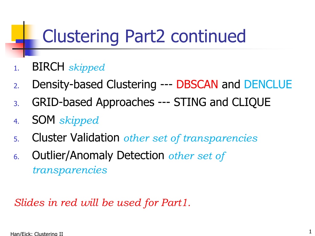
1. Clustering Part2 continued BIRCH skipped Density-based Clustering --- DBSCAN and DENCLUE GRID-based Approaches --- STING and CLIQUE SOM skipped Cluster Validation other set of transparencies Outlier/Anomaly Detection other set of transparencies 1. 2. 3. 4. 5. 6. Slides in red will be used for Part1. 1 Han/Eick: Clustering II

2. BIRCH (1996) Birch: Balanced Iterative Reducing and Clustering using Hierarchies, by Zhang, Ramakrishnan, Livny (SIGMOD 96) Incrementally construct a CF (Clustering Feature) tree, a hierarchical data structure for multiphase clustering Phase 1: scan DB to build an initial in-memory CF tree (a multi-level compression of the data that tries to preserve the inherent clustering structure of the data) Phase 2: use an arbitrary clustering algorithm to cluster the leaf nodes of the CF-tree Scales linearly: finds a good clustering with a single scan and improves the quality with a few additional scans Weakness: handles only numeric data, and sensitive to the order of the data record. 2 Han/Eick: Clustering II

3. Clustering Feature Vector Clustering Feature:CF = (N, LS, SS) N: Number of data points LS: Ni=1=Xi SS: Ni=1=Xi2 CF = (5, (16,30),(54,190)) (3,4) (2,6) (4,5) (4,7) (3,8) 10 9 8 7 6 5 4 3 2 1 0 0 1 2 3 4 5 6 7 8 9 10 3 Han/Eick: Clustering II

4. CF Tree Root CF1 CF2 CF3 CF6 B = 7 child1 child2 child3 child6 L = 6 Non-leaf node CF1 CF2 CF3 CF5 child1 child2 child3 child5 Leaf node Leaf node prev next prev next CF1CF2 CF6 CF1CF2 CF4 4 Han/Eick: Clustering II

5. Chapter 8. Cluster Analysis What is Cluster Analysis? Types of Data in Cluster Analysis A Categorization of Major Clustering Methods Partitioning Methods Hierarchical Methods Density-Based Methods Grid-Based Methods Model-Based Clustering Methods Outlier Analysis Summary 5 Han/Eick: Clustering II

6. Density-Based Clustering Methods Clustering based on density (local cluster criterion), such as density-connected points or based on an explicitly constructed density function Major features: Discover clusters of arbitrary shape Handle noise Usually one scan Need density estimation parameters Several interesting studies: DBSCAN: Ester, et al. (KDD 96) OPTICS: Ankerst, et al (SIGMOD 99). DENCLUE: Hinneburg & D. Keim (KDD 98) CLIQUE: Agrawal, et al. (SIGMOD 98) 6 Han/Eick: Clustering II

7. DBSCAN Two parameters: Eps: Maximum radius of the neighbourhood MinPts: Minimum number of points in an Eps- neighbourhood of that point NEps(p): {q belongs to D | dist(p,q) <= Eps} Directly density-reachable: A point p is directly density- reachable from a point q wrt. Eps, MinPts if 1) p belongs to NEps(q) p MinPts = 5 2) core point condition: |NEps (q)| >= MinPts q Eps = 1 cm 7 Han/Eick: Clustering II

8. Density-Based Clustering: Background (II) Density-reachable: p A point p is density-reachable from a point q wrt. Eps, MinPts if there is a chain of points p1, , pn, p1 = q, pn = p such that pi+1 is directly density-reachable from pi Density-connected p1 q p q A point p is density-connected to a point q wrt. Eps, MinPts if there is a point o such that both, p and q are density-reachable from o wrt. Eps and MinPts. o 8 Han/Eick: Clustering II

9. DBSCAN: Density Based Spatial Clustering of Applications with Noise Relies on a density-based notion of cluster: A cluster is defined as a maximal set of density-connected points Discovers clusters of arbitrary shape in spatial databases with noise Not density reachable from core point Outlier Density reachable from core point Border Eps = 1cm Core MinPts = 5 9 Han/Eick: Clustering II

10. DBSCAN: The Algorithm Arbitrary select a point p Retrieve all points density-reachable from p wrt Eps and MinPts. If p is a core point, a cluster is formed. If p ia not a core point, no points are density- reachable from p and DBSCAN visits the next point of the database. Continue the process until all of the points have been processed. 10 Han/Eick: Clustering II

11. DENCLUE: using density functions DENsity-based CLUstEring by Hinneburg & Keim (KDD 98) Major features Solid mathematical foundation Good for data sets with large amounts of noise Allows a compact mathematical description of arbitrarily shaped clusters in high-dimensional data sets Significant faster than existing algorithm (faster than DBSCAN by a factor of up to 45) But needs a large number of parameters 11 Han/Eick: Clustering II

12. Denclue: Technical Essence Influence function: describes the impact of a data point within its neighborhood. Overall density of the data space can be calculated as the sum of the influences of all data points. Clusters can be determined mathematically by identifying density attractors; object that are associated with the same density attractor belong to the same cluster Density attractors are local maximal of the overall density function. Uses grid-cells to speed up computations; only data points in neighboring grid-cells are used to determine the density for a point. 12 Han/Eick: Clustering II

13. DENCLUE Influence Function and its Gradient Example f Gaussian 2 d x y ( , ) 2 = x y ( , ) e 2 2 ( , ) d x 2 x i = N = D 2 ( ) f x e Gaussian 1 i = 2 ( , ) d x 2 x i N = D 2 ( , ) ( ) f x x x x e Gaussian i i 1 i 13 Han/Eick: Clustering II

14. Example: Density Computation D={x1,x2,x3,x4} fDGaussian(x)= influence(x1) + influence(x2) + influence(x3) + influence(x4)=0.04+0.06+0.08+0.6=0.78 2 ( , ) d x y = 2 inf ( , ) luence x y e 2 x1 x3 0.04 0.08 y x2 x4 0.6 0.06 x Remark: the density value of y would be larger than the one for x 14 Han/Eick: Clustering II

15. Example Non-Parametric DE in R Demo Rcode: setwd("C:\\Users\\C. Eick\\Desktop") a<-read.csv("c8.csv") require("spatstat") require("ppp") d<-data.frame(a=a[,1],b=a[,2],c=a[,3]) plot(d$a,d$b) w <- owin(poly=list (list(x=c(0,530,701,640,0),y=c(0,42,20,400,420)), list(x=c(320,430,310), y=c(215,200,190)),list(x=c(10,70,170,20), y=c(200,220,170, 175))) ) z<-ppp(d[,1],d[,2],window=w, marks=factor(d[,3])) plot(z) summary(z) q<-quadratcount(z, nx=12,ny=10) plot(q) den<-density(z, sigma=80) plot(den) den<-density(z, sigma=30) plot(den) den<-density(z, sigma=15) plot(den) den<-density(z, sigma=12) plot(den) den<-density(z, sigma=10) plot(den) den<-density(z, sigma=4) plot(den) documentation for function density : http://127.0.0.1:28030/library/spatstat/html/density.ppp.html 15 Han/Eick: Clustering II

16. Density Attractor 16 Han/Eick: Clustering II

17. Examples of DENCLUE Clusters 17 Han/Eick: Clustering II

18. Basic Steps DENCLUE Algorithms 1. Determine density attractors 2. Associate data objects with density attractors using hill climbing ( initial clustering) 3. Merge the initial clusters further relying on a hierarchical clustering approach (optional) 18 Han/Eick: Clustering II

19. Density-based Clustering: Pros and Cons +: can discover clusters of arbitrary shape +: not sensitive to outliers and supports outlier detection +: can handle noise + : medium algorithm complexities : finding good density estimation parameters is frequently difficult; more difficult to use than K-means. : usually, do not do well in clustering high-dimensional datasets. : cluster models are not well understood (yet) 19 Han/Eick: Clustering II

20. Chapter 8. Cluster Analysis What is Cluster Analysis? Types of Data in Cluster Analysis A Categorization of Major Clustering Methods Partitioning Methods Hierarchical Methods Density-Based Methods Grid-Based Methods Model-Based Clustering Methods Outlier Analysis Summary 20 Han/Eick: Clustering II

21. Steps of Grid-based Clustering Algorithms Basic Grid-based Algorithm Define a set of grid-cells Assign objects to the appropriate grid cell and compute the density of each cell. Eliminate cells, whose density is below a certain threshold . Form clusters from contiguous (adjacent) groups of dense cells (usually minimizing a given objective function). 1. 2. 3. 4. 21 Han/Eick: Clustering II

22. Advantages of Grid-based Clustering Algorithms fast: No distance computations Clustering is performed on summaries and not individual objects; complexity is usually O(#- populated-grid-cells) and not O(#objects) Easy to determine which clusters are neighboring Shapes are limited to union of rectangular grid- cells 22 Han/Eick: Clustering II

23. Grid-Based Clustering Methods Several interesting methods (in addition to the basic grid- based algorithm) STING (a STatistical INformation Grid approach) by Wang, Yang and Muntz (1997) CLIQUE: Agrawal, et al. (SIGMOD 98) 23 Han/Eick: Clustering II

24. STING: A Statistical Information Grid Approach Wang, Yang and Muntz (VLDB 97) The spatial area area is divided into rectangular cells There are several levels of cells corresponding to different levels of resolution 24 Han/Eick: Clustering II

25. STING: A Statistical Information Grid Approach (2) Main contribution of STING is the proposal of a data structure that can be used for many purposes (e.g. SCMRG, BIRCH kind of uses it) The data structure is used to form clusters based on queries Each cell at a high level is partitioned into a number of smaller cells in the next lower level Statistical info of each cell is calculated and stored beforehand and is used to answer queries Parameters of higher level cells can be easily calculated from parameters of lower level cell count, mean, s, min, max type of distribution normal, uniform, etc. Use a top-down approach to answer spatial data queries Clusters are formed by merging cells that match a given query description ( next slide) 25 Han/Eick: Clustering II

26. STING: Query Processing(3) Used a top-down approach to answer spatial data queries Start from a pre-selected layer typically with a small number of cells From the pre-selected layer until you reach the bottom layer do the following: For each cell in the current level compute the confidence interval indicating a cell s relevance to a given query; If it is relevant, include the cell in a cluster If it irrelevant, remove cell from further consideration otherwise, look for relevant cells at the next lower layer Combine relevant cells into relevant regions (based on grid- neighborhood) and return the so obtained clusters as your answers. 1. 2. 3. 26 Han/Eick: Clustering II

27. STING: A Statistical Information Grid Approach (3) Advantages: Query-independent, easy to parallelize, incremental update O(K), where K is the number of grid cells at the lowest level Can be used in conjunction with a grid-based clustering algorithm Disadvantages: All the cluster boundaries are either horizontal or vertical, and no diagonal boundary is detected 27 Han/Eick: Clustering II

28. Subspace Clustering Clustering in very high-dimensional spaces is very difficult High dimensional attribute spaces tend to be sparse it is hard to find any clusters It is very difficult to create summaries from clusters in very difficult This creates the motivation for subspace clustering: Find interesting subspaces (areas that are dense with respect to the attributes belonging to the subspace) Find clusters for each interesting Remark: multiple, overlapping clusters might be obtained; basically one clustering for each subspace. 28 Han/Eick: Clustering II

29. CLIQUE (Clustering In QUEst) Agrawal, Gehrke, Gunopulos, Raghavan (SIGMOD 98). Automatically identifying subspaces of a high dimensional data space that allow better clustering than original space CLIQUE can be considered as both density-based and grid- based It partitions each dimension into the same number of equal length interval It partitions an m-dimensional data space into non- overlapping rectangular units A unit is dense if the fraction of total data points contained in the unit exceeds the input model parameter A cluster is a maximal set of connected dense units within a subspace 29 Han/Eick: Clustering II

30. CLIQUE: The Major Steps Partition the data space and find the number of points that lie inside each cell of the partition. Identify the subspaces that contain clusters using the Apriori principle Identify clusters: Determine dense units in all subspaces of interests Determine connected dense units in all subspaces of interests. 30 Han/Eick: Clustering II

31. Vacation (10,000) Salary (week) 6 7 6 7 5 5 4 4 3 3 1 2 1 2 age age 0 0 20 30 40 50 60 20 30 40 50 60 = 3 Vacation 30 50 age 31 Han/Eick: Clustering II

32. Strength and Weakness of CLIQUE Strength It automatically finds subspaces of the highest dimensionality such that high density clusters exist in those subspaces It is insensitive to the order of records in input and does not presume some canonical data distribution It scales linearly with the size of input and has good scalability as the number of dimensions in the data increases Weakness The accuracy of the clustering result may be degraded at the expense of simplicity of the method Quite expensive 32 Han/Eick: Clustering II

33. Self-organizing feature maps (SOMs) Clustering is also performed by having several units competing for the current object The unit whose weight vector is closest to the current object wins The winner and its neighbors learn by having their weights adjusted SOMs are believed to resemble processing that can occur in the brain Useful for visualizing high-dimensional data in 2- or 3-D space 33 Han/Eick: Clustering II

34. References (1) R. Agrawal, J. Gehrke, D. Gunopulos, and P. Raghavan. Automatic subspace clustering of high dimensional data for data mining applications. SIGMOD'98 M. R. Anderberg. Cluster Analysis for Applications. Academic Press, 1973. M. Ankerst, M. Breunig, H.-P. Kriegel, and J. Sander. Optics: Ordering points to identify the clustering structure, SIGMOD 99. P. Arabie, L. J. Hubert, and G. De Soete. Clustering and Classification. World Scietific, 1996 M. Ester, H.-P. Kriegel, J. Sander, and X. Xu. A density-based algorithm for discovering clusters in large spatial databases. KDD'96. M. Ester, H.-P. Kriegel, and X. Xu. Knowledge discovery in large spatial databases: Focusing techniques for efficient class identification. SSD'95. D. Fisher. Knowledge acquisition via incremental conceptual clustering. Machine Learning, 2:139-172, 1987. D. Gibson, J. Kleinberg, and P. Raghavan. Clustering categorical data: An approach based on dynamic systems. In Proc. VLDB 98. S. Guha, R. Rastogi, and K. Shim. Cure: An efficient clustering algorithm for large databases. SIGMOD'98. A. K. Jain and R. C. Dubes. Algorithms for Clustering Data. Printice Hall, 1988. 34 Han/Eick: Clustering II

35. References (2) L. Kaufman and P. J. Rousseeuw. Finding Groups in Data: an Introduction to Cluster Analysis. John Wiley & Sons, 1990. E. Knorr and R. Ng. Algorithms for mining distance-based outliers in large datasets. VLDB 98. G. J. McLachlan and K.E. Bkasford. Mixture Models: Inference and Applications to Clustering. John Wiley and Sons, 1988. P. Michaud. Clustering techniques. Future Generation Computer systems, 13, 1997. R. Ng and J. Han. Efficient and effective clustering method for spatial data mining. VLDB'94. E. Schikuta. Grid clustering: An efficient hierarchical clustering method for very large data sets. Proc. 1996 Int. Conf. on Pattern Recognition, 101-105. G. Sheikholeslami, S. Chatterjee, and A. Zhang. WaveCluster: A multi-resolution clustering approach for very large spatial databases. VLDB 98. W. Wang, Yang, R. Muntz, STING: A Statistical Information grid Approach to Spatial Data Mining, VLDB 97. T. Zhang, R. Ramakrishnan, and M. Livny. BIRCH : an efficient data clustering method for very large databases. SIGMOD'96. 35 Han/Eick: Clustering II