Understanding Similarity and Cluster Analysis in Business Intelligence and Analytics
Explore the concept of similarity and distance in data analysis, major clustering techniques, and algorithms. Learn how similarity is essential in decision-making methods and predictive modeling, such as using nearest neighbors for classification and regression. Discover (dis)similarity functions, nearest neighbor classifiers, and considerations like majority vote and cross-validation in predictive modeling.
Download Presentation

Please find below an Image/Link to download the presentation.
The content on the website is provided AS IS for your information and personal use only. It may not be sold, licensed, or shared on other websites without obtaining consent from the author. Download presentation by click this link. If you encounter any issues during the download, it is possible that the publisher has removed the file from their server.
E N D
Presentation Transcript
Business Intelligence and Analytics: Similarity and cluster analysis Session 7
Agenda Similarity and distance Introduction to cluster analysis Major clustering techniques and algorithms Validation of Clusterings Case Study
Similarity and distance Similarity is at the core of many DM methods o If two things are similar in some ways, they often share o other characteristics as well Some business cases o Use similarity for classification and regression o Group similar items together into clusters o Provide recommendations to people (Amazon, Netflix) o Reasoning from similar cases (medicine, law)
(Dis)similarity functions Typically, distances between data objects are used for the determination of similarity Euclidean distance between two p-dimensional data objects i and j | x x |2+ | x x |2+ + | x x |2 i1 j1 i2 j2 d(i, j) = ip jp Manhattan distance (more robust) d(i, j) =| xi1 xj1|+| xi2 xj2|+ +| xip xjp| Minkowski distance (generalization) q d(i, j) = (| xi1 xj1| +| xi2 xj2| + +| x x | ) q q 1/ q ip jp Special distance functions for binary, nominal and ordinal scaled variables
Nearest neighbors for predictive modeling Idea of similarity in predictive modeling: Given a new example whose target variable we want to predict, we scan through all the training examples and choose several that are the most similar to the new example. Then we predict the new example s target value, based on the nearest neighbors (known) target values Classification: look for the nearest neighbors and derive target class for new example Regression: derive target value from the mean or median of the neighbors
Nearest neighbor in classification (1/2) Majority vote How many neighbors? Also consider the distance to vary the influence of the neighbors
Nearest neighbor in classification (2/2) Nearest neighbor classifiers follow very specific boundaries 1-NN strongly tends to overfit (k is a complexity parameter!) Use cross-validation or nested holdout testing
Issues with nearest neighbor methods Intelligibility Decisions can be explained along the contributions of the neighbors: The movie Billy Elliot was recommended based on your interest in Amadeus, The Constant Gardener and Little Miss Sunshine NN methods lack of specific decision models Dimensionality Having too many/irrelevant attributes may confuse distance calculations course of dimensionality Solution 1: Feature selection Solution 2: Inject domain knowledge in distance calculation Computational Efficiency Querying the database for prediction can be very expensive
Agenda Similarity and distance Introduction to cluster analysis Major clustering techniques and algorithms Validation of Clusterings Case Study 10
What is cluster analysis? (1/2) Clustering is the process of grouping data into classes or cluster so that objects within a cluster have high similarity in comparison to one another, but are very dissimilar to objects in other clusters. Cluster = collection of data objects that are similar to each other Two main purposes: Discovery of overall distribution patterns and interesting correlations among data attributes Data reduction: a cluster can be treated collectively as one group in many applications Clustering is an example of unsupervised learning
Typical applications of clustering Help marketers discover distinct groups in their customer databases and characterize customer groups based on purchasing patterns Derive plant and animal taxonomies in biology, categorize genes with similar functionality Identification of groups of automobile insurance policy holders with a high average claim cost Classify documents on the web for information discovery Gain insight into the distribution of data Preprocessing step for other tasks such as classification
Typical requirements of clustering in data mining (1/2) Many cluster algorithms work well on small low dimensional data sets and numerical attributes In large data sets, algorithms must be able to deal with the following circumstances: Scalability (e.g., handle millions of data objects) Different types of attributes (e.g., binary, nominal, ordinal) Discover clusters with arbitrary shape (not all clusters are shaped like a circle)
Typical requirements of clustering in data mining (2/2) Domain knowledge required to determine input parameters and evaluate results Deal with noisy data outliers can massively influence the clustering Insensitivity to the order of input records High dimensionality Interpretability and usability
Agenda Similarity and distance Introduction to cluster analysis Major clustering techniques and algorithms Validation of Clusterings Case Study
Major clustering techniques and algorithms (1/2) A large number of clustering algorithm exists The choice of cluster algorithm depends on the type of data available the particular purpose and application The user has to choose the clustering technique carefully domain knowledge required Clustering algorithms compare data objects regarding to their similarity or dissimilarity
Major clustering techniques and algorithms (2/2) selectionand executionof clustering validation ofclustering results selectionof dataobjects andvariables interpretation ofresults target dataset database resultsof clustering validated results information aboutstructure (adaptedfrom Halkidi et al. (2001)) Criteria for appropriate selection of clustering algorithm (Tan et al. (2009)): - type and structure of clustering - type and definition of clusters - features of the data set - number of data objects and variables - representation of results
Partitioning based clustering Given a database of ? objects, a partitioning method constructs ? partitions of the data (k n) Each partition represents a cluster. Result: the data is classified into k groups Each group must contain at least one object Each object must belong to exactly one group General approach Create an initial partitioning Improve the partitioning by an iterative relocation technique, i.e., move data objects from one group to another Criteria: objects in the same group are close to each other, whereas objects of different clusters are far apart
Partitioning based clustering: k-means (1/3) Input: number of clusters k and a database containing ? objects Output: set of k clusters that minimizes the squared-error criterion Method: arbitrarily choose k objects as the initial cluster centers; repeat (re)assign each object to the cluster to which the object is the most similar, based on the mean value of the objects in the cluster; update the cluster means, i.e., calculate the mean value of the objects or each cluster; until no change; i= 1 k E = | p m | i p C i p = data point mi = mean of Cluster Ci Squared-error criterion:
Partitioning based clustering: k- means (2/3) Example: a b c General remarks: works well when clusters are compact clouds and well separated scalable and efficient in large data sets often terminates at local optimum ( random initial partitioning!) mean must be defined (e.g., not suitable for categorical attributes) sensitive to noisy and outlier data ( mean calculation) 20
Partitioning based clustering: k-means (3/3) Interactive demonstration of k-means algorithm: http://home.dei.polimi.it/matteucc/Clustering/tutorial_html/AppletKM.html
Partitioning based clustering: k-medoids instead of taking the mean value as a reference, the medoid is used medoid = most centrally located object in a cluster main idea: Find k clusters in ? objects by first arbitrarily determining a representative object (= medoid) for each cluster each remaining object is clustered with the medoid to which it is the most similar the medoids are iteratively replaced by one of the non- medoids as long as the quality of clustering is improved (i.e., the actual square-error ? is reduced) k-medoids is more robust than k-means processing is more costly than the k-means
Hierarchical based clustering (1/2) Creates a hierarchical decomposition of a set of data objects Two main approaches: Agglomerative approach (bottom up): start with each object as a separate group, then successively merge groups until a certain termination condition holds Divisive approach (top-down): start with all objects in one cluster, then successively split up into smaller clusters until a certain termination condition holds Han et. al Main disadvantage: Once a merge or split is done, it can never be undone, i.e., erroneous decisions cannot be corrected
Hierarchical based clustering (2/2) Measures for distances between two clusters: Minimum distance between two data points Maximum distance between two data points Mean distance, i.e., distance between the mean of the clusters Average distance, (the avg of all single distances) The user can specify the desired number of clusters as a termination condition Critical decision: where to split or merge groups? Risk of low-quality clusters No well scaling since the decision of merge or split needs to examine and evaluate a good number of objects or clusters
Hierarchical based clustering: Chameleon (1/3) explores dynamic modeling of the neighborhood in hierarchical clustering Karypis et al. counteracts disadvantages of common hierarchical algorithms two clusters are merged if the interconnectivity and closeness between two clusters are highly related to the internal interconnectivity and closeness of objects within the clusters general approach: use a graph partitioning algorithm to cluster the data objects into a large number of relatively small temporary clusters combine or merge sub-clusters with an agglomerative hierarchical cluster algorithm
Hierarchical based clustering: Chameleon (2/3) K-nearest neighbor graph each vertex represents a data object two vertices are connected if one object is among the k-most similar objects of the other Karypis et al.
Hierarchical based clustering: Chameleon (3/3) The neighborhood radius of an object is determined by the density of the region in which this object resides In a dense region, the neighborhood is defined narrowly In a sparse region, it is defined more widely The edge of a dense region tends to weigh more than that of a sparse region Han et. al
Density-based clustering continues growing the given clusters as long as the density (i.e., the number of objects or data points) in the neighborhood exceeds some threshold discovers clusters with arbitrary shapes due to not using the distance between data objects for clustering DBSCAN algorithm (simplified): check the neighborhood of each point in the database find satisfying neighborhoods merge satisfying neighborhoods which are connected Han et. al
Grid-based clustering: STING (1/2) Divide the object space into a finite number of cells that form a grid structure Main advantage: fast processing time, which is typically independent of the number of data objects Typical example: STING (STatistical INformation Grid) Spatial area is divided into rectangular cells Hierarchical structure Statistical information (mean, max, min, ) regarding the attributes in each grid cell are pre-computed and stored Han et. al
Grid-based clustering: STING (2/2) Advantages: Grid structure facilitates parallel processing and incremental updating The method is very efficient: STING goes through the database once to compute the statistical parameters The query processing time is much smaller due to the small number of grid cells at the lowest level General remarks: The quality of STING depends on the granularity of the lowest level of the grid structure The shapes of the resulting clusters are either horizontal or vertical, no diagonal boundary is detected 30
Agenda Similarity and distance Introduction to cluster analysis Major clustering techniques and algorithms Validation of Clusterings Case Study 31
Validation of clusterings Visualize results of cluster analysis ( exploratory data analysis) Internal measures define the quality of a clustering based on the given data set cluster cohesion / cluster separation e.g., Davies-Bouldin index External measures compare the results of a clustering with established structure or information (e.g. manual clustering by an expert) Relative measures are derived from internal and external measures compare several clusterings regarding a given hypothesis
Davies-Bouldin index internal measure for validation of clusterings compare variation of data objects within the clusters i and j [s(??), s(??)] to distance between the clusters i and j ??)] calculation for every pair i,j : [d(??, ??? is small when distances between clusters are large and variations in clusters are small ( good clustering ) overall calculation: take the maximum ??? for every instance of k : calculate overall index
Clustering tendency Does the given data set tend to natural clusters? Test on spatial randomness of the data set Hopkins statistic Generate ? objects in ?-dimensional data space randomly Mark ? objects in the original data set randomly Find nearest neighbors for both sets and add distances p u + i ud i=1 H = i p p d d w i=1 i=1 i H 0.5 data set is randomly distributed H > 0.5 data set tends to clusters
Determination of the number of clusters Many cluster algorithms require the number k of clusters Idea: approximate determination of k A data set is clustered several times with varying k For every clustering, (wk) is calculated (wk) is visualized, indicating possible values of k w k : use the squared-error criterion or an internal measure like the Davies-Bouldin index as function ? and search for a local optimum as an indication for an appropriate number k K isapplicationspecific visualizationnecessary
References Provost, F.; Fawcett, T.: Data Science for Business; Fundamental Principles of Data Mining and Data- Analytic Thinking. O Reilly, CA 95472, 2013. Carlo Vecellis, Business Intelligence, John Wiley & Sons, 2009 Eibe Frank, Mark A. Hall, and Ian H. Witten : The Weka Workbench, M Morgan Kaufman Elsevier, 2016. Jason Brownlee, Machine Learning Mastery With Weka, E-Book, 2017
