Enhancing Hydrogeophysical Data Integration with the Prediction-Focused Approach
The Prediction-Focused Approach (PFA) offers a unique Bayesian method for integrating and interpreting hydrogeophysical data. Unlike traditional methods, PFA focuses on forecasting target variables rather than model parameters, utilizing an ensemble of prior models to establish a direct relationship between data and forecasts. This method involves steps like constructing a realistic conceptual model, reducing problem dimensionality through PCA, and solving the inverse problem using Gaussian regression. By applying PFA, researchers can efficiently generate samples of posterior distributions for improved data interpretation and integration.
- Hydrogeophysics
- Data Integration
- Prediction-Focused Approach
- Bayesian Method
- Hydrogeological Interpretation

Download Presentation

Please find below an Image/Link to download the presentation.
The content on the website is provided AS IS for your information and personal use only. It may not be sold, licensed, or shared on other websites without obtaining consent from the author. Download presentation by click this link. If you encounter any issues during the download, it is possible that the publisher has removed the file from their server.
E N D
Presentation Transcript
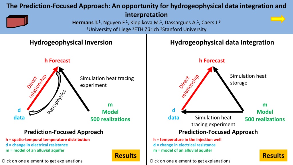
The Prediction-Focused Approach: An opportunity for hydrogeophysical data integration and interpretation Hermans T.1, Nguyen F.1, Klepikova M.1, Dassargues A.1, Caers J.3 1University of Liege 2ETH Z rich 3Stanford University Hydrogeophysical Inversion Hydrogeophysical data Integration Hydrogeophysical Inversion Hydrogeophysical data Integration h Forecast h Forecast h Forecast h Forecast Direct relationship Direct relationship Simulation heat storage Simulation heat tracing experiment Simulation heat storage Simulation heat tracing experiment Petrophysics m Model 500 realizations m Model 500 realizations m m d data d data d d Model Model Simulation heat tracing experiment data data Simulation heat tracing experiment Prediction-Focused Approach h = temperature in the injection well d = change in electrical resistance m = model of an alluvial aquifer 500 realizations 500 realizations Prediction-Focused Approach Prediction-Focused Approach Prediction-Focused Approach h = spatio-temporal temperature distribution d = change in electrical resistance m = model of an alluvial aquifer Results Results Results Results Click on one element to get explanations Click on one element to get explanations
Home slide Home slide The prediction-focused approach The prediction focused approach (PFA) is a Bayesian method, that differs from other Bayesian methods developed in hydrogeology and hydrogeophysics because its likelihood function is formulated in a reduced dimension space based on target variables (prediction/forecast) and not on model parameters. PFA relies on an ensemble of prior models whose size is limited, to derive a direct relationship between data variables and forecast variables, avoiding a full explicit inversion to generate the posterior distribution of the forecast. The methodology can be divided in 6 steps 1) Construction of a realistic conceptual model of the experiment (prior models) including all sources of uncertainty (parameter distribution, spatial heterogeneity, structural uncertainty, boundary conditions, etc.). From this prior, n realizations or samples are 2) Forward modeling of the forecast (inversion or integration) and the data variables for each realization. Both data and forecast are high-dimensional. In the case of hydrogeophysical inversion, data variables are obtained after petrophysical transformation of the forecast variables 3) Reduction of the size of the problem through application of principal component analysis (PCA) on both data and forecast (inversion or integration) to retain only their first components. This provides two reduced sets. 4) Linearization of the relationship between data and forecast variables (inversion or integration) in the reduced dimension space through canonical correlation analysis (CCA). The resulting linear relationships are independent. 5) Solving the inverse problem in the reduced dimension space using a Gaussian regression process. 6) The posterior distribution being multivariate Gaussian, it is straightforward to generate samples in the reduced dimension space. By back transformation of CCA and PCA, it is possible to generate samples of the posterior distribution in the original space (inversion or integration).
Home slide Home slide Definition of the prior PFA is based on a realistic definition of the prior model. The prior model aims at identifying the variation of model parameters from background knowledge. This includes broad information on the geological context and specific information on the study site acquired in previous experiments. Based on this background knowledge, we define realistically their prior distribution, i.e. the value they are expected to take according to the current knowledgeof the site. Parameters Fixed/Variable Value Mean of log10K (m/s) Variable U[-4 -1] Variance log10K (m/s) Variable U[0.05 1.5] Range (m) Variable U[1 10] Anisotropy ratio Variable U[0.5 10] Orientation Variable U[- /4 - /4] From this prior, we generate several plausible models of the subsurface with sequential Gaussian simulations, by randomly sampling values of the uncertain parameters. This constitutes the prior set of models, each modelbeing one possiblerealizationof the subsurface. Porosity Variable U[0.05 0.40] Gradient (%) Variable U[0 0.167] log10K (m/s) upper layer Fixed 10-5 Longitudinal dispersivity (m) Fixed 1 Transverse dispersivity (m) Fixed 0.1 Model parameter uncertainty (K) Spatial uncertainty (variogram model) Boundary condition uncertainty (gradient) Solid thermal conductivity (W/mK) Fixed 3 Water thermal conductivity (W/mK) Fixed 0.59 Solid specific heat capacity (J/kgK) Fixed 1000 Water specific heat capacity (J/kgK) Fixed 4189 1 realization from the prior
Home slide Home slide Heat tracing experiment The field experiment is a forced gradient heat tracing experiment monitored with cross-borehole electrical resistivity tomography. The forced gradient is in the direction of the natural one so that it enables to fasten groundwater flow without affecting the flow direction encountered in natural conditions. The use of geophysical methods enables to collect spatially distributed data, informing on the spatial heterogeneity of the aquifer. The location of the monitoring network is such that the temperature is still at a level easily detectable by ERT, but its spatial distribution is already affected by the heterogeneity of the aquifer. The experiment is simulated for each realization of the prior to compute the spatio-temporal distribution of temperature at the location of the ERT panel. This constitutes the forecast for the hydrogeophysical inversion. The ERT data is simulated through a petrophysical relationship.This constitutes the data for both cases.
Home slide Home slide Spatio-temporal distribution of temperature The simulated for each realization of the prior to compute the spatio-temporal distribution of temperature at the location of the ERT panel. heat tracing experiment is The panel is divided in a grid of 26 x 28 cells (cell size of 0.25 m x 0.25 m) and the temperature simulated at 6 different time-steps, leading to a total of 4368 dimensions. distribution is The dimension can be reduced using PCA. In this case, the 8 first dimensions represent about 90% of the total variance It is transformed into time-lapse ERT data using a petrophysical relationship and ERT forward model. The hydrogeophysical inversion is to derive the spatio-temporal distribution of temperature corresponding observed field data. aim of PFA in the to
Home slide Home slide Petrophysics and ERT data The petrophysical relationship relates the change in water electrical conductivity due to the change in temperature induced by the heat tracing experiment The dimension of the data can also be reduced using PCA. In this case, the 10 first dimensions represent more than 95% of the total variance ERT data are then simulated for 410 different electrode configurations for six time-steps (2460 dimensions) The temperature distribution is transformed into a resistivity distribution using a petrophysical relationship = m (25 T) 1 + f,T f f,25 mf = 0.0194 C-1
Home slide Home slide Direct relationship between temperature distribution and ERT Canonical correlation analysis (CCA) is used to transform the relation between the reduced data and forecast variables into a set of independent linearized relationships. This process provides 8 independent linear relationships in the reduced dimension space. For the first dimensions, the correlation is very high and then decreases. The black line represents where the observed data lies in the reduced dimension space. If it lies outside of the prior (red point), it means that the prior is not consistent with field observations. The eight relationships being independent and linear, they can be analytically inverted (Gaussian regression) to derive the mean and standard deviation of the posterior distribution of the forecast in the reduced dimension space. The only condition is that the prior distribution must be Gaussian, what can be ensured through histogram transform. This posterior distribution can be sampled and back-transformed to get the posterior distribution of the sought prediction (in high dimension space).
Home slide Home slide Prediction of the temperature distribution during the heat tracing experiment Once the posterior distribution in the low dimension space is known, we can randomly draw samples from it. Those samples are in the reduced dimensional space, but they can be back-transformed in the original space. This process is very fast since all computations are already done (forward hydrogeological simulations). We therefore obtain relatively quickly the posterior distributions of temperature in the aquifer during the experiment. 3 samples show a heat plume limited to the bottom part of the aquifer and divided in 2 different parts with a lower temperature in the middle of the section. Most uncertainty is related to the level of temperature change and the smallscale temperaturedistribution. Direct measurements in the aquifer offer independent measurements to validate the proposed predictions. The posterior distribution of temperature changes at those two positions shows that the temporal behavior of the tracer is very well caught by ERT data. The reduction of uncertainty compared to the prior is large but the uncertainty on the temperature variations remains relatively high. The limit of detection of ERT in this experiment was estimated at about 1.5 C (Hermans et al., 2015). The level of uncertainty derived with PFA thus seems relatively coherentwith the limitationof the methoditself.
Home slide Home slide Long-term Heat Storage The final objective of the study is to assess the ability of an alluvial aquifer to store thermal energy and restore it in a later stage. This corresponds to the theoreticalconceptof an Aquifer Thermal Energy Storage(ATES) system. Summer The process is simulated through a heat storage scenario for all models of the prior. During 30 days, heated water is continuously injected in a well at a rate of 3 m /h. The temperature of the injected water is 10 C above the background temperature. At the end of the 30-day period, water is extracted from the well at the same rate of 3 m /h. The change in temperature of the pumped water compared to the initial value in the aquifer (i.e., before injection) is recorded for another 30-day period. The aim is to be able to predict the thermal energy that can be recovered during the pumping phase using the heat tracing experimentthrough PFA. Heat pump Water table Warm well Cold well The thermal energy recovery corresponding to the simulated ATES system can be estimated using the temperature of the extracted water. The simulation is limited in time to avoid considering changing boundary conditions with time. Similarly, a rate of 3 m /h allows to reduce the size of the investigatedzone.
Home slide Home slide Heat storage capacity of the aquifer The heat storage experiment is simulated for each realization of the prior to compute the curve of temperature at the well during the pumping phase of the experiment. The simulation is divided into 30 period of 1 day (30 dimensions). Given the range of variations of model parameter as described by the prior, the range of temperature during the pumping phase spans a very large range of possible value, from almost zero recovered energy to a consequent amount of energy recovery. The green curve illustrates the prediction made for a model calibrated deterministically. The aim of PFA in the hydrogeophysical integration is to derive the spatio- temporal distribution of temperature corresponding to data observed during the heat tracing experiment The forecast of heat storage is much simpler than heat tracing (less dimension) and the two first dimensions after PCA represent more than 99% of the variance.
Home slide Home slide Direct relationship between ERT and heat storage capacity Canonical correlation analysis (CCA) is used to transform the relation between the reduced data and forecast variables into a set of independent linearized relationships. This process provides 2 independent linear relationships in the reduced dimension space. The black line represents where the observed data lies in the reduced dimension space. If it lies outside of the prior (red point), it means that the prior is not consistent with field observations. Scenario 1 1 day In this case, we compare two scenarios. Scenario 1 considers only the first day of heat tracing. Scenario 2 considers the whole heat tracing experiment. Scenario 2 5 days We see that Scenario 2 provides more information than Scenario 1, because the correlation of the linear relationship is larger. This means that the posterior distribution will be more reliable.
Home slide Home slide Prediction of the heat storage capacity using the heat tracing experiment Once the posterior distribution in the reduced dimension space is known, we can randomly draw samples from it. Those samples are in the reduced dimensional space, but they can be back- transformedin the original space. Scenario 1 1 day This procedure is very fast since all computations are already done (forward hydrogeological simulations). We therefore obtain relatively quickly the posterior distributions of temperature in the aquifer during the pumping phase. The calculated posterior distribution of the change of temperature at the well indicates that the potential for heat storage on the field site is relatively low, in accordance with the deterministic solution. Most samples of the posterior have a rapid decrease in temperature once the pumping phase starts. The uncertainty in the prediction is relatively low compared to the prior distribution of temperature at the well. Scenario 2 5 days The 5-day experiment is more informative and should improve the prediction. The position of the 90% quantile suggests that the probability of the aquifer to have a higher heat storage capacity is slightlyincreased consideringthe 5-day experiment.
The Prediction-Focused Approach: An opportunity for hydrogeophysical data integration and interpretation Hermans T.1, Nguyen F.1, Klepikova M.1, Dassargues A.1, Caers J.3 1University of Liege, Urban and Environmental Engineering 2ETH Z rich, Earth Sciences 3Stanford University, Geological Sciences
Regularized deterministic solutions lack geological realism Quantitative interpretation is difficult Hydrogeological integration is complex True distribution X Deterministic inversion X Too smooth Z Z Amplitude underestimation Resolution-dependent petrophysics Estimation of reservoir properties difficult (ex: saturation, temperature)
Changing the paradigm Forecast = Quantitative geophysical model or Hydrogeological prediction from geophysics
Determination of a statistical relationship using a training data set 500 Realizations h Forecast Objective Establish a linear relationship In a reduced dimension space m d Model data Forecast h 500 Realizations of the alluvial aquifer 500 Realizations dobs data d 16
An example of geophysical inversion a heat tracing experiment Data = Change in resistance with time 410 measurements Forecast = Change in temperature with time 728 cells 17
Building the prior Parameters Fixed/Variable Value Mean of log10K (m/s) Variable U[-4 -1] 500 realizations = prior models Variance log10K (m/s) Variable U[0.05 1.5] Range (m) Variable U[1 10] Anisotropy ratio Variable U[0.5 10] Orientation Variable U[- /4 - /4] Porosity Variable U[0.05 0.40] Gradient (%) Variable U[0 0.167] log10K (m/s) upper layer Fixed 10-5 Hydrogeological forward model simulating the tracing experiment (temperature distribution Longitudinal dispersivity (m) Fixed 1 Transverse dispersivity (m) Fixed 0.1 Solid thermal conductivity (W/mK) Fixed 3 Water thermal conductivity (W/mK) Fixed 0.59 Petrophysical relationship to derive the resistivity distribution and simulation of ERT data Solid specific heat capacity (J/kgK) Fixed 1000 Water specific heat capacity (J/kgK) Fixed 4189
Dimension reduction and sampling Principal component analysis (10 dimensions in the data, 8 in the forecast) Canonical correlation analysis to linearize the relationship
An example of geophysical integration : predicting heat storage Data = Change in resistance with time 410 measurements Forecast = Heat storage Temperature of extracted water 21
Dimension reduction and prediction PCA (10 dimensions in the data, 2 in the forecast) Direct prediction of long-term heat storage from geophysical heat tracing data High correlations in CCA Low storage capacity of the aquifer
Conclusion PFA to invert geophysical data PFA to integrate geophysics in hydrogeological predictions Uncertainty quantification Definition of the prior is the most important step Fast prediction (no explicit inversion) Can be fully parallelized


 and Validation")