Solving NP-Complete Problems Using Backtracking and Branch-and-Bound
The journey through NP-Complete problems involves proving complexity, utilizing backtracking for intelligent exhaustive search, and adopting branch-and-bound for optimization. These techniques offer strategies to tackle intricate challenges efficiently, elevating your status as a problem solver within your project team.

Download Presentation

Please find below an Image/Link to download the presentation.
The content on the website is provided AS IS for your information and personal use only. It may not be sold, licensed, or shared on other websites without obtaining consent from the author. Download presentation by click this link. If you encounter any issues during the download, it is possible that the publisher has removed the file from their server.
E N D
Presentation Transcript
NP-Complete Problems and how to go-on with them Data Structures and Algorithms A.G. Malamos References: Algorithms, 2006, S. Dasgupta, C. H. Papadimitriou, and U . V . Vazirani Introduction to Algorithms, Cormen, Leiserson, Rivest & Stein
intro Y ou are the junior member of a seasoned project team. Y our current task is to write code for solving a simple-looking problem involving graphs and numbers. What are you supposed to do? If you are very lucky , your problem will be among the half-dozen problems concerning graphs with weights (shortest path, minimum spanning tree, maximum flow , etc.), that we have solved in this book. Even if this is the case, recognizing such a problem in its natural habitat -grungy and obscured by reality and context requires practice and skill. It is more likely that you will need to reduce your problem to one of these lucky ones- or to solve it using dynamic programming or linear programming. But the remaining vast expanse is pitch dark: NP-complete. What are you to do? You can start by proving that your problem is actually NP-complete. Often a proof by generalization (recall the discussion on page 270 and Exercise 8.10) is all that you need; and sometimes a simple reduction from 3SAT or ZOE is not too diffcult to find. This sounds like a theoretical exercise, but, if carried out successfully , it does bring some tangible rewards: now your status in the team has been elevated, you are no longer the kid who can't do, and you have become the noble knight with the impossible quest. But, unfortunately , a problem does not go away when proved NP-complete. The real question is, What do you do next?
Intelligent exhaustive search Backtracking Backtracking is based on the observation that it is often possible to reject a solution by looking t just a small portion of it. For example, if an instance of SAT contains the clause (x1 + x2) then all assignments with x1 = x2 = 0 (i.e., false) can be instantly eliminated. To put it differently , by quickly checking and discrediting this partial assignment, we are able to prune a quarter of the entire search space. A promising direction, but can it be systematicallyexploited? Here's how it is done. Consider the Boolean formula (w, x,y,z) specified by the set of Clauses (w +x+y+z)*(w+x )*(x+y )*(y+z )*(z+w )*(w +z ) We will incrementally grow a tree of partial solutions. We start by branching on any one variable, say w The partial assignment w = 0, x = 1 violates the clause (w+x ) and can be terminated, thereby pruning a good chunk of the search space. We backtrack out of this dead-end and continue our explorations at one of the two remaining active nodes.
backtracking More abstractly , a backtracking algorithm requires a test that looks at a subproblem and quickly declares one of three outcomes: 1. Failure: the subproblem has no solution. 2. Success: a solution to the subproblem is found. 3. Uncertainty .
Branch and Bound The same principle can be generalized from search problems such as SAT to optimization problems. For concreteness, let's say we have a minimization problem; maximization will follow the same pattern. As before, we will deal with partial solutions, each of which represents a subproblem, namely, what is the (cost of the) best way to complete this solution? And as before, we need a basis for eliminating partial solutions, since there is no other source of efficiency in our method. To reject a subproblem, we must be certain that its cost exceeds that of some other solution we have already encountered. But its exact cost is unknown to us and is generally not efficiently computable. So instead we use a quick lower bound on this cost.
Branch & Bound TSP How can we lower-bound the cost of completing a partial tour [a,S,b]? Many sophisticated methods have been developed for this, but let's look at a rather simple one. The remainder of the tour consists of a path through V -S, plus edges from a and b to V-S. Therefore, its cost is at least the sum of the following: 1. The lightest edge from a to V-S. 2. The lightest edge from b to V-S. 3. The minimum spanning tree of V S. Reminder: Min Spanning tree is a subgraph that is a tree and connects all the vertices together
Approximation algorithms In an optimization problem we are given an instance I and are asked to find the optimum solution the one with the maximum gain if we have a maximization problem like INDEPENDENT SET, or the minimum cost if we are dealing with a minimization problem such as the TSP. For every instance I, let us denote by OPT(I) the value (benefit or cost) of the optimum solution. It makes the math a little simpler (and is not too far from the truth) to assume that OPT(I) is always a positive integer . More generally, consider any minimization problem. Suppose now that we have an algo- rithmA for our problem which, given an instance I, returns a solution with value A(I). The approximation ratio of algorithm A is defined to be The goal is to keep ratio very low, however how can we calculate the optimal since this is the parameter we are asking to determine? This solution is feasible into convenient problems where the optimal value is known but we are looking for the optimal way to get it! (ex optimal path with a given cost bound)
Local search heuristics Our next strategy is inspired by an incremental process of introducing small mutations, trying them out, and keeping them if they work well. This paradigm is called local search and can be applied to any optimization task. Here's how it looks for a minimization problem.
Local Optima Heuristics-Simulated annealing The method of simulated annealing redefines the local search by introducing the notion of a random T. Simulated annealing is inspired by the physics of crystallization. When a substance is to be crystallized, it starts in liquid state, with its particles in relatively unconstrained motion. Then it is slowly cooled, and as this happens, the particles gradually move into more regular configurations. This regularity becomes more and more pronounced until finally a crystal lattice is formed.
Local Optima Heuristics-Simulated annealing