Sustainable Agroecosystem Management Stakeholder Meeting

The Stakeholder Advisory Committee Meeting on April 2, 2021, focused on discussing important topics like farmer adaptations to climate risks, ecosystem services, economic modeling, and policy assessments. Led by a team of experts and stakeholders, the meeting aimed to explore the right set of policies for achieving sustainable and resilient agroecosystem management while balancing agricultural production with critical ecosystem services. Participants actively engaged in discussions and evaluations to address the impact of climate change on farmer decision-making and identify policies to promote sustainability and resilience.

Download Presentation

Please find below an Image/Link to download the presentation.
The content on the website is provided AS IS for your information and personal use only. It may not be sold, licensed, or shared on other websites without obtaining consent from the author. Download presentation by click this link. If you encounter any issues during the download, it is possible that the publisher has removed the file from their server.
E N D
Presentation Transcript
Stakeholder Advisory Committee Meeting April 2, 2021
Agenda 11:00 Welcome and fill out evaluation survey! 11:15 - Review farmer survey infographic (Robyn/Jason) 11:30 - Land use/adaptation modeling (Robyn/Elena) 12:00 - Ecosystem services water quality (Kai) 12:15 Break 12:45 - Economic modeling with COVID-19 results (YY) 1:15 - Scenario discussions national/regional policy triggers (Alan) 1:50 Final Thoughts 2:00 Wrap up 2
Photo credit: Blanchard Demo Farms Introductions Research Team Dr. Robyn Wilson project director Dr. Elena Irwin land use modeling Dr. Aaron Wilson climate modeling Stakeholder Advisory Team Kirk Merritt Ohio Soybean Council Dr. Larry Antosch Ohio Farm Bureau Dr. Dennis Todey USDA Midwest Climate Hub Dr. Carl Zulauf OSU Emeritus Ag Policy Steve Emery Nutrien Ag Solutions Mark Apelt Becks Hybrid Nate Andre Andre Farms Luke Crumley Ohio Corn & Wheat Jeff Goetz The Andersons Gail Hesse National Wildlife Federation Kevin Elder Farmer Matthew Adams Ag Credit Photo credit: Midwest Cover Crops Council Dr. Kaiguang Zhao services modeling Dr. Yongyang Cai economic modeling Greg LaBarge - extension Dr. Bryan Mark state climatologist Dr. Alan Randall economic modeling Jason Cervenec educ & outreach Dr. Kristi Lekies - evaluator Dr. Mary Doidge behavioral modeling Post-docs/GRAs: Hugh Walpole, Ziqian Gong, Ziyu Guo, Shelby Taber, Mackenzie Jones Photo credit: Seneca County Conservation District 3
Overall research question In the face of climate risks and uncertainties that influence farmer adaptations What is the right set of policies and programs to achieve sustainable and resilient agroecosystem management that balances agricultural production with critical ecosystem services? 4
What is the impact of climate and farmer decision making on ecosystem services? Downscaled climate modeling Farmer adaptation survey Ecosystem services model Given this spatially explicit understanding, what are the expected regional economic outcomes? Dynamic, regional economic model What policies might best promote sustainability and resilience? Optimal policy assessment 5
Evaluations! https://osu.az1.qualtrics.com/jfe/form/SV_1GDlLIo822Oo0pT
Farmer Survey Infographic Review and provide suggestions
Land Use & Adaptation Updates on the extent to which we can connect future adaptations to changes in land use
If you remember from last time What are agricultural land use and crop rotation trends in our study region? How much do they vary over space and over time? How are they correlated with observable land management practices (based on remotely sensed data) What s reasonable for us to assume in our model scenarios in terms of crop-land management correlations? How might these correlations change over time? 13
Agricultural Land Use (percent of total land area) Lower Maumee 60% 50% 40% Percent 30% 20% 10% 0% 2008 2009 2010 2011 2012 2013 2014 2015 2016 2017 2018 corn soy wheat pasture Source: USDA Cropland Data Layer (CDL) https://www.nass.usda.gov/Research_and_Science/Cropland/Release/ 14
Crop Rotations (percent of total cropland) Lower Maumee 70 60 50 40 Percent 30 20 10 0 2008-2010 2011-2013 2014-2016 2017-2018 All soy All corn Corn/soy Wheat/soy Corn/Soy/Wheat Source: USDA Cropland Data Layer (CDL) https://www.nass.usda.gov/Research_and_Science/Cropland/Release/ overlaid with historical field boundaries approximations 15
Lower Maumee Use of no & reducted till over time Use of cover crops over time Use of high & moderate residue over time 40% 100% 100% 95% 35% 90% 85% 30% Percent of acres Percent of acres 85% 70% 25% 80% 20% 75% 55% 70% 15% 40% 65% 10% 60% 25% 5% 55% 10% 50% 0% 2009 2010 2011 2012 2013 2014 2015 2016 2017 2018 Year 2009 2010 2011 2012 2013 2014 2015 2016 2017 2018 Year 2009 2010 2011 2012 2013 2014 2015 2016 2017 2018 Year Soybeans Small Grains Corn 16 Source: Conservation Technology Information Center: https://www.ctic.org/OpTIS_tabular_query (combined OpTIS categories)
Trends Similar adoption rates of each practices across crops and watersheds Higher adoption of no till & reduced till Moderate adoption of high & medium residue Low adoption of cover crops Dominant rotation is corn/soy increasing corn/soy over time with other rotations decreasing or constant declining cover crops with soy over time in Lower Maumee 17
Trends Feedback from you on future trends (from Dec mtg) Beans will continue to increase, corn/wheat will continue to decrease (due to markets, labor) Negative drivers of cover crops Corn Availability and cost of seed Rented land (which will continue to increase) Climate/weather (double cropping/longer season varieties, wet conditions, late harvest) Positive drivers of cover crops Beans (which will continue to go up) H2OH (for a few years) Climate/weather (dry conditions, early harvest) 18
2 Land use modeling (DRFEWS) Land management/adaptations modeling (NIFA) 1 Change my rotation to allow for double cropping Install more tile drainage on my farm Change my insurance coverage (Yield/Revenue, Increase/Decrease) Increase my use of no-till/conservation tillage Enroll more of my land in conservation programs; ____________acres Invest in new or additional irrigation on my farm I would not make any of these changes Econometric model: Use historical land use data to estimate land use change parameters associated with land rents and conversion costs for each land use transition. Conditional on allocations of cropland to corn, soy, wheat, and conservation how will this influence land management/ adaptations? Land uses = cropland (corn, soy, wheat, conservation, specialty), pasture, forest, wetland, urban For each management practice, probability of adoption as function of: Planting & harvesting dates Rainfall Conservation payments Farmer attributes Construct rents using historical data = estimated rents for each land use given output prices, land characteristics, etc. Proxy for conversion costs using soil quality variables and other observable physical, geographic features at county level Likelihood of Adoption: Two-stage model: (1) Adopt 0/1; (2) Conditional on adopting, which practices? (1) determined more by ind behavioral + farm size (2) is determined more by econ or climate conditions + farm size Output from LU change model: Set of land use transition equations that predict land use change given output and input prices, physical land characteristics, regional population and GDP, etc. We are trying to estimate likelihood of adaptation conditional on land use/crop allocations using the NIFA survey data? Farmer attributes that enter choice model and that are sometimes significant depending on adaptation: From CGE model: Given total cropland allocation in a given year, allocation of land to specific crops and conservation land given individual supply elasticities (from DRFEWS survey) and price changes Farm size, Years farming (highly correlated w age), Crop insurance (yes/no - Varies by state, e.g., MI has low uptake levels), Concern about CC impacts, Negative experience w CC, Conservationist identity, Education, Family succession) We also know for a typical year: crop allocations, crop rotation, conservation, tillage practices, cover crops, tile drainage, amount of rented land, amount of crop insurance Output from CGE model: Allocation of land to specific crops, conservation, pasture, and non-ag (forest, wetland, urban) uses 19
Linking Land Use to Land Management Trying to link crops/land use to adaptations/land mgmt. We added crops/baseline land use to the adaptation models and found limited effects Crops, hay, conservation, livestock as land use categories Found only an effect of baseline conservation on more land in retirement Re-think the model specification? Combine land use categories differently combine livestock with hay, pull wheat out from crops and put with conservation or hay, consider using crop rotations Remove the heterogeneity (identity, concern, etc) and location variables focus first on CE variables and land use, then add in observable IVs (farm size, age, educ) Working on these new analyses May have to consider a random parameters specification due to DV structure, machine learning for the two-stage decision, other analytic approaches? 20
Potential effects across analyses Do nothing Variables Increase no till More tile Retire more land Greater chance of weather changes More likely Less likely Later harvest date Less likely Later planting date More likely More likely Greater rainfall Less likely More likely Less likely Greater cons payments More likely Less likely More baseline acres in hay More baseline acres in conservation More likely More baseline acres in corn/soy/wheat Larger farm size More likely More likely Less likely Higher education More likely More likely Less likely 21
How might you expect land use/crop rotations to vary with tillage practices, tiling, and land retirement over time? What about other practices? Double cropping? Changes in insurance coverage? Irrigation? 22
Ecosystem Services How to handle the water quality piece
Overview of this sub-task Quantify changes in ecosystem services under possible future scenarios Climate Land use Management practice Model-based assessments using the SWAT watershed model A model is as good as the assumptions put into it The quality of model outputs are as good as the quality of input data No attempt made to improve the SWAT model itself 24
Typical water quality metrics: a quick example Surface runoff Sediment yield P concentrations & load Particulate P Dissolved P N concentration & load 25
Climate and land-use scenarios: Relatively straightforward 26
Lower Maumee: prediction driven purely by changing climate 27
Management Scenarios: borrowed from Martin et al. (2021) 1 No point source discharge 100% point source removal source contribution 100% removal of P from manure (baseline N application maintained) source contribution 25% less P fertilizer applied source contribution 2 No manure application 3 25% P rate reduction 4 Broadcast P All fertilizer is broadcast without incorporation management effect 5 Broadcast and incorporated P All fertilizer is broadcast with incorporation management effect All P fertilizer is subsurface applied (99% below top 1 cm of soil) management effect All manure applied in fall management effect All manure applied in spring management effect 6 Subsurface applied P 7 Fall manure 8 Spring manure 9 Fall and spring manure Manure applied half in spring and half in fall management effect Fertilizer and manure P applications decreased by 50% and subsurface applied P in the fall Cover crops on 100% of cropland management effect Controlled drainage (or drainage water management) in 100% of tile drained areas by 10 Rate, placement, and timing 11 Cereal rye cover crop 12 Controlled drainage 13 Headwater wetlands Wetlands in all subbasins receive 50% of flow management effect 28
Management Scenarios: borrowed from Martin et al. (2021) 58% cover crops + 50% subsurface placement of P + 78% buffer strips | scenario, random implementation 58% cover crops + 50% subsurface placement of P + 78% buffer strips| scenario, targeted implementation 14 In-field + Buffers (Random) 15 In-field + Buffers 60% cover crops + 68% subsurface placement of P + 50% buffer strips| scenario, survey data, targeted implementation 58% cover crops + 50% subsurface placement of P + 78% wetlands |scenario, targeted implementation 50% cover crops + 60% subsurface placement of P + 50% no-tillage +15% controlled drainage| scenario, targeted implementation 16 Likely Adoption of In-field +Buffers 17 In-field + Wetlands 18 In-field + Controlled drainage 29
Economic Model Presentations of model with COVID-19 results
Global Disruption Due to Covid-19: Evaluating the Potential Impact on the Ohio Economy Yongyang Cai et al. April 2, 2021 32
Schematic 33
Schematic 34
Infection and Mortality Infection Seasonality Vaccine (availability and effectiveness) Economic activities Behavior change over time from learning Mortality Decreasing over time fromlearning Seniors have a higher mortalityrate 35
Labor and Health Workers provide labor and has disutility from working Seniors and Other do not work Infected patients do not work More infected, less uninfected workers or work time Some lose theirjobs Some look after those infected patients Some are not willing to work More infected, less labor productivity in each sector 36
Impact of COVID-19 to Ohio 831,067 confirmed infection by January 18,2021 10,283 death from COVID-19 by January 18,2021 Ohio GDP dropped 3.2% between the third quarter of 2019 and the third quarter of2020 The November 2020 unemployment rate in Ohio: 5.7% Lower salary Lesshealthy 38
Scenarios Baseline: All Ohioans will get their COVID-19 vaccination by August 2021 Vaccine has 90% effectiveness (even if there are mutations) More economic activities lead to a higher infection rate If 25% Ohioans refuseCOVID-19 vaccine 25% of Americans in a new poll from Monmouth University said they are still unwilling to be vaccinated. If there were noCOVID-19 39
No COVID-19 44
Designing Scenarios What global to local drivers and potential policies/programs should we be thinking about for our region?
Scenarios provide the Context for modeling Alternative Policies and Strategies Scenarios are representations of o The status quo o The trends and drivers that will help shape the future Our Region is Nested in the Nation and the World o This has implications: Scenarios must be multi-part, addressing possible future configurations of the world, the nation, and our region Scenarios must be plausible why model the absurd? But they should stretch the bounds of plausibility we can t be complacent about the future Scenarios must be internally consistent some configurations of our regional future are inconsistent with some national and global futures 46
Scenarios provide the Context for modeling Alternative Policies and Strategies (continued) Scenarios are representations of o The status quo o The trends and drivers that will help shape the future Policies are distinguished from scenarios o Policies are pro-active efforts to (i) mitigate problems that might emerge given a scenario and/or (ii) open-up opportunities for betterment o Our time horizon runs until the year 2100 During that time, stresses may emerge if trends and drivers are permitted to run These stresses may depend on the particular scenario, e.g. a fossil fuels intensive scenario might accelerate climate impacts, which might trigger abrupt policy changes o Today we plan to discuss policies that might lie just over the horizon, but may become highly relevant by year 2100 47
Our scenarios are layered, to reflect this nesting Looking forward, several different futures are possible for the world, the nation, and our region Global Trends and Drivers Regional Trends and Drivers National Trends and Drivers 48
Toward Global Scenarios Shared Socioeconomic Pathways (SSPs) Low for Mitigation High Socioeconomic Challenges SSP4: Inequality SSP1: Sustainability SSP2: Middle of the Road SSP3: Regional Rivalry SSP5: Fossil-Fueled Low Socioeconomic Challenges for Adaptation High 49
Higher Sustainability, Best Case Climate Global Trends and Drivers Renewable energy dominates (e.g., no fossil fuel subsidies) Aggressive carbon mitigation, water quality enhancement Land, soil conservation, biodiversity, habitat incentives International subsidies for participation by low-income countries Moderate economic growth in industrialized countries Low income countries lag behind Poor have inadequate access to resources Social cohesion degrades Conflict/unrest increasingly common Moderate economic growth in industrialized countries? High economic growth in low-income countries? Poor have adequate access to resources? Social cohesion improves? Conflict less common? More people Not so well off vs BAU Business As Usual Fewer people Better off vs BAU Fossil fuels dominate (e.g., fossil fuel subsidies) Carbon deregulated (e.g., no carbon tax) Water quality benign neglect (e.g., minimal regulation) Deregulated land clearing & use, no conservation incentives Increased migration driven by water scarcity Lower Sustainability, Worst Case Climate 50 50


")
")


")
")


")
")