Optimization Techniques for Minimization Problems


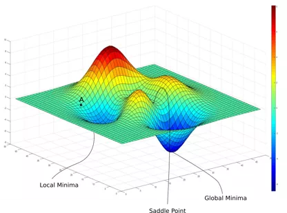
Minimization problems: from
easy to hard to insanely hard.

Easy
Hard

Find Local optimum.
function of 1 variable
Find Local optimum.
function of N variables
Find global optimum.
function of N variables

Minimization problem

Easy
Hard

Find Local optimum.
function of 1 variable
The “bisection” approach to
finding single minimum:
The most efficient version: golden
section.
•
Keeps on bracketing the root by dividing the
initial interval and choosing the half where the
minimum is by comparing value of the function
“up hill” and “down hill”. Continues until the
convergence criteria are met, e.g.
|x
n+1
– x
n
| < TOL (assuming x ~1. )
•
Linear convergence. Robust but slow.
•
https://www.youtube.com/watch?v=VBFuqglVW
3c
Newton’s method for finding local
minimum.
Motivation: utilize more information
about the function. Hope to be faster.
Simplest derivation
If F(x) -> minimum at x
m,
then F’(x
m
) = 0.
Solve for F’(x
m
) = 0 using Newton’s for root finding.
Remember, for Z(x) = 0, Newton’s iterations are x
n+1
= x
n
+ h,
where h = -Z(x
n
)/Z’(x
n
)
Now, substitute F’(x) for Z(x)
To get h = -F’(x
n
)/F’’(x
n
)
So, Newton’s iterations for minimization are: x
n+1
= x
n
- F’(x
n
)/F’’(x
n
)
Rationalize Newton’s Method
Let’s Taylor expand F(x) around it minimum, x
m
:
F(x) = F(x
m
) + F’(x
m
)(x – x
m
) + (1/2)*F’’(x
m
)(x – x
m
)
2
+ (1/3!)*F’’’(x
m
)(x – x
m
)
3
+ …
Neglect higher order terms for |x – x
m
| << 1, you must start
with a good initial guess anyway.
Then F(x) ≈ F(x
m
)+ F’(x
m
)(x – x
m
) + (1/2)*F’’(x
m
)(x – x
m
)
2
But recall that we are expanding around a minimum, so F’(x
m
) =0.
Then F(x) ≈ + F(x
m
) + (1/2)*F’’(x
m
)(x – x
m
)
2
So, most functions look like a parabola around their local minima!
Newton
’
s Method = Approximate the
function with a parabola, iterate.
X
0
X
m
Newton
’
s Method
Newton
’
s Method
Newton
’
s Method
Newton
’
s method. More informative derivation.
N
e
w
t
o
n
’
s
m
e
t
h
o
d
f
o
r
f
i
n
d
i
n
g
m
i
n
i
m
u
m
h
a
s
q
u
a
d
r
a
t
i
c
(
f
a
s
t
)
c
o
n
v
e
r
g
e
n
c
e
r
a
t
e
f
o
r
m
a
n
y
(
b
u
t
n
o
t
a
l
l
!
)
f
u
n
c
t
i
o
n
s
,
b
u
t
m
u
s
t
b
e
s
t
a
r
t
e
d
c
l
o
s
e
e
n
o
u
g
h
t
o
s
o
l
u
t
i
o
n
t
o
c
o
n
v
e
r
g
e
.
Example
Newton’s: convergence to local minimum.
•
If x
0
is chosen well (close to the min.), and the
function is close to a quadratic near minimum,
the
convergence is fast, quadratic
. E.g: |x0 –
x
m
| < 0.1,
•
Next iteration: |x1– x
m
| < (0.1)
2
•
Next: |x2– x
m
| < ((0.1)
2)2
= 10
-4
•
Next: 10
-8
, etc.
Newton’s: convergence to local minimum.
•
If x
0
is chosen well (close to the min.), and the function is
close to a quadratic near minimum, the
convergence is fast,
quadratic
. E.g: |x0 – x
m
| < 0.1,
•
Next iteration: |x1– x
m
| < (0.1)
2
•
Next: |x2– x
m
| < ((0.1)
2)2
= 10
-4
•
Next: 10
-8
, etc.
•
In general, convergence to the minimum is NOT guaranteed
(run-away, cycles, does not converge to x
m
, etc. Sometimes,
convergence may be very poor even for “nice looking”,
smooth functions! )
•
Combining Newton’s with slower, but more robust methods
such as “golden section” often helps.
•
No numerical method will work well for truly ill-conditioned
(pathological) cases. At best, expect significant errors, at
worst – completely wrong answer!
Choosing stopping criteria
•
The usual: |x
n+1
– x
n
| < TOL, or, better
•
|x
n+1
– x
n
| < TOL*|x
n+1
+ x
n
|/2
to ensure that
the given TOL is achieved for the
relative
accuracy.
•
Generally,
TOL ~ sqrt(ε
mach
) or larger if full
theoretical precision is not needed. But not
smaller.
•
TOL can not be lower because, in general F(x) is
quadratic around the minimum x
m
, so when you
are h < sqrt(ε
mach
) away from x
m
,
|F(x
m
) –
F(x
m
+h)| < ε
mach,
and you can no longer
distinguish between values of F(x) so close to the
min.
The stopping criterion: more details
•
To be more specific, assume root bracketing (golden
section). We must stop iterations when |F(x
n
) – F(x
m
)| ~
ε
mach*
|F(x
n
) |, else we can no longer tell F(x
n
) from F(x
m
)
and further iterations are meaningless.
•
Since |F(x
n
) – F(x
m
)| ≈ |(1/2)*F’’(x
m
)(x
n
– x
m
)
2
| , we get
for this smallest |(x
n
– x
m
)| ~ sqrt(ε
mach
)* sqrt(|2F(x
n
) /
F’’(x
m
) |) = sqrt(ε
mach
)* sqrt(|2F(x
n
) / F’’(x
n
) |) =
sqrt(ε
mach
)*|x
n
|*sqrt(
|2F(x
n
) /(x
n
2
F’’(x
n
)) |
) .
•
For many functions the quantity in green
| | ~1,
which
gives us the rule from the previous slide:
stop when |x
n+1
– x
n
| < sqrt(ε
mach
)* |x
n+1
+ x
n
|/2
Explore various minimization problems, from easy to insanely hard, and learn about finding global and local optima using approaches like bisection, Newton's method, and rationalization. Discover efficient methods such as the golden section and iterative approximation with Newton's method for optimizing functions with multiple variables.

Download Presentation

Please find below an Image/Link to download the presentation.
The content on the website is provided AS IS for your information and personal use only. It may not be sold, licensed, or shared on other websites without obtaining consent from the author. Download presentation by click this link. If you encounter any issues during the download, it is possible that the publisher has removed the file from their server.
E N D
Presentation Transcript
Minimization problems: from easy to hard to insanely hard. Find global optimum. function of N variables Find Local optimum. function of N variables Find Local optimum. function of 1 variable Easy Hard
Minimization problem Find Local optimum. function of 1 variable Easy Hard
The bisection approach to finding single minimum:
The most efficient version: golden section. Keeps on bracketing the root by dividing the initial interval and choosing the half where the minimum is by comparing value of the function up hill and down hill . Continues until the convergence criteria are met, e.g. |xn+1 xn| < TOL (assuming x ~1. ) Linear convergence. Robust but slow. https://www.youtube.com/watch?v=VBFuqglVW 3c
Newtons method for finding local minimum. Motivation: utilize more information about the function. Hope to be faster.
Simplest derivation If F(x) -> minimum at xm, then F (xm) = 0. Solve for F (xm) = 0 using Newton s for root finding. Remember, for Z(x) = 0, Newton s iterations are xn+1 = xn + h, where h = -Z(xn)/Z (xn) Now, substitute F (x) for Z(x) To get h = -F (xn)/F (xn) So, Newton s iterations for minimization are: xn+1 = xn - F (xn)/F (xn)
Rationalize Newtons Method Let s Taylor expand F(x) around it minimum, xm: F(x) = F(xm) + F (xm)(x xm) + (1/2)*F (xm)(x xm)2+ (1/3!)*F (xm)(x xm)3+ Neglect higher order terms for |x xm| << 1, you must start with a good initial guess anyway. Then F(x) F(xm)+ F (xm)(x xm) + (1/2)*F (xm)(x xm)2 But recall that we are expanding around a minimum, so F (xm) =0. Then F(x) + F(xm) + (1/2)*F (xm)(x xm)2 So, most functions look like a parabola around their local minima!
Newtons Method = Approximate the function with a parabola, iterate. X0 Xm
Newtons method. More informative derivation. Newton s method for finding minimum has quadratic (fast) convergence rate for many (but not all!) functions, but must be started close enough to solution to converge.
Newtons: convergence to local minimum. If x0 is chosen well (close to the min.), and the function is close to a quadratic near minimum, the convergence is fast, quadratic. E.g: |x0 xm | < 0.1, Next iteration: |x1 xm | < (0.1)2 Next: |x2 xm | < ((0.1)2)2 = 10-4 Next: 10-8, etc.
Newtons: convergence to local minimum. If x0 is chosen well (close to the min.), and the function is close to a quadratic near minimum, the convergence is fast, quadratic. E.g: |x0 xm | < 0.1, Next iteration: |x1 xm | < (0.1)2 Next: |x2 xm | < ((0.1)2)2 = 10-4 Next: 10-8, etc. In general, convergence to the minimum is NOT guaranteed (run-away, cycles, does not converge to xm, etc. Sometimes, convergence may be very poor even for nice looking , smooth functions! ) Combining Newton s with slower, but more robust methods such as golden section often helps. No numerical method will work well for truly ill-conditioned (pathological) cases. At best, expect significant errors, at worst completely wrong answer!
Choosing stopping criteria The usual: |xn+1 xn | < TOL, or, better |xn+1 xn | < TOL*|xn+1 + xn |/2 to ensure that the given TOL is achieved for the relative accuracy. Generally, TOL ~ sqrt( mach) or larger if full theoretical precision is not needed. But not smaller. TOL can not be lower because, in general F(x) is quadratic around the minimum xm, so when you are h < sqrt( mach) away from xm,|F(xm) F(xm+h)| < mach, and you can no longer distinguish between values of F(x) so close to the min.
The stopping criterion: more details To be more specific, assume root bracketing (golden section). We must stop iterations when |F(xn) F(xm)| ~ mach*|F(xn) |, else we can no longer tell F(xn) from F(xm) and further iterations are meaningless. Since |F(xn) F(xm)| |(1/2)*F (xm)(xn xm)2| , we get for this smallest |(xn xm)| ~ sqrt( mach)* sqrt(|2F(xn) / F (xm) |) = sqrt( mach)* sqrt(|2F(xn) / F (xn) |) = sqrt( mach)*|xn|*sqrt(|2F(xn) /(xn2F (xn)) |) . For many functions the quantity in green | | ~1, which gives us the rule from the previous slide: stop when |xn+1 xn | < sqrt( mach)* |xn+1 + xn |/2