Understanding Small Set Expansion in Johnson Graphs
In this detailed piece, Subhash Khot, Dor Minzer, Dana Moshkovitz, and Muli Safra explore the fascinating concept of Small Set Expansion in Johnson Graphs. The Johnson Graph is defined as a representation where nodes are sets of size K in a universe of size N, and two sets are connected if they intersect in L elements. The article delves into the Johnson Graph as a slice of a Noisy Hypercube and its application in Direct Product Testing. Additionally, the expansion of sets in a d-regular graph and the concept of Small Set Expansion are explored with examples like the Noisy Hypercube and the limitations of the Johnson Graph as a Small Set Expander. The discussion extends to the Zoom-in family, highlighting the challenges of identifying Small Set Expanders and the implications of pseudorandomness within set families.
Download Presentation

Please find below an Image/Link to download the presentation.
The content on the website is provided AS IS for your information and personal use only. It may not be sold, licensed, or shared on other websites without obtaining consent from the author. Download presentation by click this link. If you encounter any issues during the download, it is possible that the publisher has removed the file from their server.
E N D
Presentation Transcript
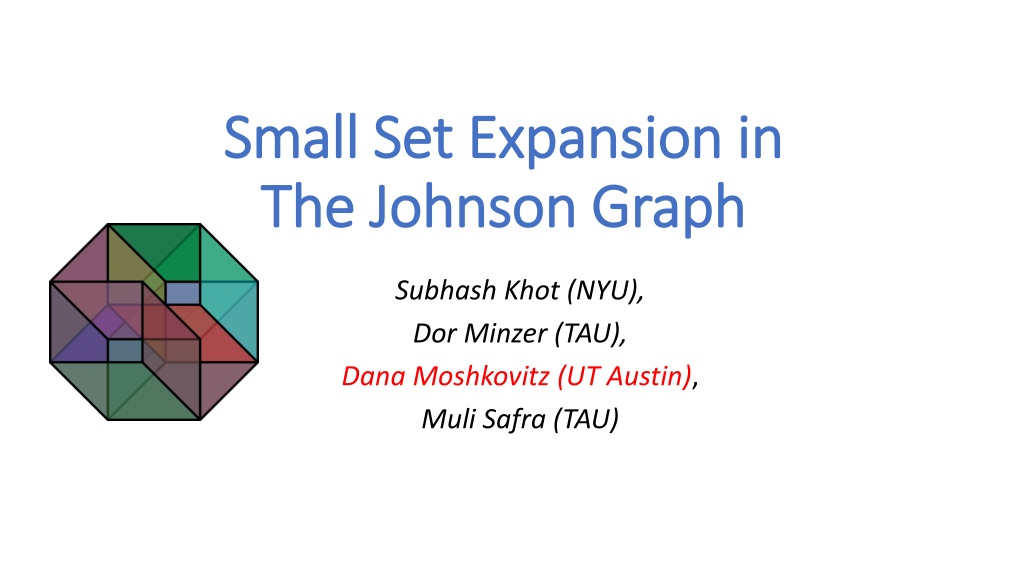
S Small Set Expansion in mall Set Expansion in The Johnson Graph The Johnson Graph Subhash Khot (NYU), Dor Minzer (TAU), Dana Moshkovitz (UT Austin), Muli Safra (TAU)
The Johnson Graph Definition (Johnson graph): The nodes are sets of size K in a universe of size N (typically, K<<N). Two sets are connected if they intersect in L elements (typically, L= (K)).
The Johnson Graph As Slice of Noisy Hypercube Noisy hypercube graph (variant): the vertices are strings in {0,1}N. There is an edge between x and y if they differ on N coordinates. Johnson graphs are slices of noisy hypercube: restrict to strings with K ones. Edges correspond to intersection of size L=(1- )K. N 1 0 0 1 0 0 0 1 0 0
The Johnson Graph Underlies Direct Product Testing Direct Product Test: Two players supposedly agree on N bits. A verifier picks at random two sets S,T [N], |S|=|T|=k, |S T|=L. The verifier sends S to one player, T to the other player. Each player is supposed to send the K bits indicated by their set. The verifier checks that the answers on L common bits are the same. S S T T
Expansion Let G=(V,E) be a d-regular graph. The expansion of S V is (S) = |E(S,V-S)| / (d|S|). Small Set Expander: (S) 1- for all S of size < |V|. S Examples: The noisy hypercube is a small set expander by hypercontractivity. The Johnson graph is not a small set expander (K<<N, L/K large).
Johnson Graph - Not Not Small Set Expander Dictator The Zoom-in family: Pick an element x and consider the family S of all sets that contain x. |S|/|(Nk)| (K/N) [small for K<<N] (S) 1 (L/K) [much smaller than 1 for constant L/K]. Rough Statement of Main Theorem: Except for dictator like families , all small families S in the Johnson graph have (S) 1-o(1).
Unlike Dictator Dfn: A family S of sets is (r, )-pseudorandom if for all R [N], |R| r, |PA R(A S) - PA(A S) | Examples: Dictator is not pseudorandom: for S = {A that contains x} take R={x}, so PA R(A S)=1, while PA(A S) K/N. A sufficiently large random family S is pseudorandom with high probability. Main Theorem: Let S be of fraction at most and (r, )- pseudorandom. For sufficiently large N (as a function of K and 1/ ), (S)>1 (L/K)r 2O(r)poly( ) o(1).
Approach ? ? The proof is via spectral analysis. Let J be the transition matrix of the Johnson graph. Let F be the indicator of a small pseudorandom family. Want to show <F,JF> is small. ? ? J F
The Johnson transition matrix J has K+1 eigenspaces; the i th has eigenvalue roughly (L/K)i. Level Picture Main Lemma: Small pseudorandom families F= i Fi concentrated on upper levels, i.e., i r|Fi|22<0.01|F|22. K K-1 r r-1 0 From Main Lem To Main Thm: Let F be small pseudorandom. Write F= i Fi with Fi in i th space. <F,JF> = i <Fi,JFi> i>r (L/K)i|Fi|22 (L/K)r|F|22.
The Eigenspaces A We say that a function F from sets of size K to the reals is of degree i if there exists f from sets of size i to the reals such that: F(A) = I A,|I|=i f(I). For example: F(A) = does A contain x? is of degree 1: take f({y})= does y=x? . Lemma: Let Si be the space of functions of degree i that are orthogonal to the functions of degree i-1. Then Si is an eigenspace of J with eigenvalue (L/K)i.
The Johnson transition matrix J has K+1 eigenspaces; the i th corresponds to degree i; has eigenvalue roughly (L/K)i. Level Picture Main Lemma: Small pseudorandom families F= i Fi concentrated on upper levels, i.e., i r|Fi|22<0.01|F|22. K K-1 r ... 1 0 For simplicity, we ll prove that F is not almost entirely in one level i, i.e., |Fi|22<0.99|F|22 Zoom-in/Dictators
Fourth Moment Lemma: Let N be sufficiently large. Let F be of fraction and (r, )-pseudorandom with F=F0+ +FK where Fi is in the i th eigenspace. Then for i=0, ,r, we have EA[Fi(A)4] 2O(i) EA[Fi(A)2] + o(1). F not almost entirely on one level 0 i r: Assume on way of contradiction that |Fi|22 0.99|F|22=0.99 . Then F(A) Fi(A) for all but at most 0.01 fraction of A, and since F is a set of fraction we have EA[Fi(A)4] EA[F(A)4]=EA[F(A)2] EA[Fi(A)2] , which contradicts the Fourth Moment Lemma. (More generally, Fourth Moment Lemma implies EA[Fi(A)2] 2O(i) 1/4 + o(1) for i=0, ,r, which implies the main lemma)
The Main Technical Difficulty Fourth Moment Lemma: Let N be sufficiently large. Let F be of fraction and (r, )-pseudorandom with F=F0+ +FK where Fi is in the i th eigenspace. Then for i=0, ,r, we have EA[Fi(A)4] 2O(i) EA[Fi(A)2] + o(1). Write Fi(A)= I A,|I|=i f(I). EA[Fi(A)4]=EA[ I1,I2,I3,I4 A,|Ij|=i f(I1)f(I2)f(I3)f(I4)]. I2 How to bound correlations?? I1 I4 I3
For simplicity, assume i=3 and consider third moments. Fix the intersection pattern (How many elements in I1 I2 I3? How many in I1c I2 I3? ). For simplicity, focus on the pattern below. Cauchy-Schwarz & Restrict technique: Ex1,x2,x3,x4[f({x1,x2,x3})f({x1,x2,x4})f({x2,x3,x4})] Ex2,x3,x4[Ex1[f({x1,x2,x3})f({x1,x2,x4})]f({x2,x3,x4})] Ex2,x3,x4[Ex1[f({x1,x2,x3})2]1/2 Ex1[f({x1,x2,x4})2]1/2f({x2,x3,x4})] Ex2,x4[Ex3[Ex1[f({x1,x2,x3})2]1/2f({x2,x3,x4})]Ex1[f({x1,x2,x4})2]1/2] Ex2,x4[Ex3,x1[f({x1,x2,x3})2]1/2Ex3[f({x2,x3,x4})2]1/2Ex1[f({x1,x2,x4})2]1/2] Ex2[Ex3,x1[f({x1,x2,x3})2]1/2Ex4[Ex3[f({x2,x3,x4})2]1/2Ex1[f({x1,x2,x4})2]1/2]] Ex2[Ex3,x1[f({x1,x2,x3})2]1/2Ex4,x3[f({x2,x3,x4})2]1/2Ex4,x1[f({x1,x2,x4})2]1/2] Ex2[Ex3,x1[f({x1,x2,x3})2]Ex4,x3[f({x2,x3,x4})2]]1/2Ex2,x4,x1[f({x1,x2,x4})2]1/2 (maxx2Ex3,x1[f({x1,x2,x3})2]Ex2,x4,x3[f({x2,x3,x4})2]Ex2,x4,x1[f({x1,x2,x4})2])1/2 (maxx2Ex3,x1[f({x1,x2,x3})2])1/2 Ex1,x2,x3[f({x1,x2,x3})2] Can be shown to be proportional to: (maxxEB[Fi(B {x})2])1/2 EA[Fi(A)2] I2 Upper bounded by O( ) from pseudorandomness I1 I3
