Risk Management: Methods, Procedures, and Techniques

This unit delves into the methods, procedures, and techniques used by risk managers to minimize risks within a firm. It covers risk identification, measurement, treatment, and the tools of risk management. Understanding and managing risks are crucial for organizations to mitigate potential losses and undesirable events.

Download Presentation

Please find below an Image/Link to download the presentation.
The content on the website is provided AS IS for your information and personal use only. It may not be sold, licensed, or shared on other websites without obtaining consent from the author. Download presentation by click this link. If you encounter any issues during the download, it is possible that the publisher has removed the file from their server.
E N D
Presentation Transcript
UNIT UNIT- - 2 2 RISK MANAGEMENT RISK MANAGEMENT 1
2.1 Introduction 2.1 Introduction This unit focuses on the methods, procedures and techniques used by the risk manager so as to minimize the risk occur in a firm. Once we understand that risk always exist with a firm or human being activities, managers should take different measure to avoid or reduce these losses or undesired events. 2
2.2 Definition of Risk Management 2.2 Definition of Risk Management Risk Management is the identification, measurement, and treatment of property, liability, and personnel pure-risk exposures. It involves the application of general management concepts to a specialized area. In requires the drawing up of plans, the organizing of material and individual for the undertaking, the maintaining of activity among personnel for the objectives, involved, the unifying and coordinating all the activities and efforts, and finally the controlling these activities. 3
2.3 Risk Management Process 2.3 Risk Management Process 1: Risk identification The loss exposures of the business or family must be identified. Risk identification is the first and perhaps the most difficult function that the risk manager or administrator must perform. Failure to identify all the exposures of the firm or family means that the risk manager will have no opportunity to deal with these unknown exposures intelligently. 4
2.3 Risk Management Process (Cont.) 2.3 Risk Management Process (Cont .) 2: Risk Measurement:- After risk identification, the next important step is the proper measurement of the losses associated with these exposures. This measurement includes a determination of: the probability or chance that the losses will occur The impact the losses would have upon the financial affairs of the firm or family should they occur. The ability to predict the losses that will actually occur during the budget period. The measurement process is important because it indicates the exposures that are most serious and consequently most in need of urgent attention. It also yields information needed in risk treatment. 5
2.3 Risk Management Process (Cont.) 2.3 Risk Management Process (Cont .) 3: Tools of Risk Management Once the exposures has been identified and measured the various tools of risk management should be considered and a decision made with respect to the best combination of tools to be used in attacking the problems. These tools include. avoiding the risk reducing the chance that the loss will occur or reducing its magnitude if it does occur transferring risk to some other party, and retaining or bearing the risk internally 6
2.3 Risk Management Process (Cont.) The third alternative includes, but not limited to the purchase of insurance. In selecting the proper tool or combination of tools the risk manager must establish the cost and other consequences of using each tool or combination of tools. He/she must also consider the present financial condition/position/ of the firm or family, it s over all policy with reference to risk management and its specific objectives. 7
2.3 Risk Management Process (Cont.) 2.3 Risk Management Process (Cont .) 4: Implementation: After deciding among the alternative tools of risk treatment the risk manager must implement the decisions made. If insurance is to be purchased for example, establishing proper coverage, obtaining reasonable rates, and selecting the insurer are part of the implementation process. 8
2.3 Risk Management Process (Cont.) 2.3 Risk Management Process (Cont .) 5: Controlling/monitoring: The results of the decisions made and implemented in the first four steps must be monitored to evaluate the wisdom of those decisions and to determine whether changing conditions suggest different solutions. 9
2.4 Objectives of Risk Management 2.4 Objectives of Risk Management Mere survival:- to exist as a business enterprise as a going concern Peace of mind:- to avoid mental and physical strain of uncertainty of a person Lower risk management costs and thus higher profits Fairly stable earnings:-to eliminate the fluctuating nature of earnings due to fluctuating losses. Little or no interruptions of operations Continued growth Satisfaction of the firm s sense of social responsibility or desire for a good image/creating good will on society/value maximization Satisfaction of externally imposed obligations. 10
2 2. .5 5 Risk Risk Identification Identification Risk identification is the process by which a business systematically and continually identifies property, liability, and personnel exposures as soon as or before they emerge. The risk manager tries to locate the areas where losses could happen due to a wide range of perils. Unless the risk manager identifies all the potential losses confronting the firm, he or she will not have any opportunity to determine the best way to handle the undiscovered risks. 11
2.5 Risk Identification (Cont) 2.5 Risk Identification (Cont ) To identify all the potential losses the risk manager needs first a checklist of all the losses that could occur to any business. Second, he or she needs a systematic approach to discover which of the potential losses included in the checklist are faced by his/her business. The risk manager may personally conduct this two-step procedure or may rely upon the services of an insurance agent, broker, or consultant. After the checklist is developed, the second step is to discover and describe the types of losses faced by a particular business. Because most business is complex, diversified, dynamic operations, a more systematic method of exploring all facets of the specific firm is highly desirable. 12
2.5 Risk Identification (Cont) 2.5 Risk Identification (Cont ) Seven methods that have been suggested are: 1. the risk analysis questionnaire 2. the financial statement method 3. the flow-chart method 4. on-site inspection 5. planned interactions with other departments 6. statistical records of past losses 7. analysis of the environment 13
2 2. .5 5 Risk Risk Identification Identification (Cont (Cont ) ) No single method or procedure of risk identification is free of weaknesses or can be called foolproof. The strategy of management must be to employ that method or combination of method that best fits the situation at the hand. The choice depends on: The nature of the business The size of the business The availability of in house expertise, etc. 14
2.5 Risk Identification (Cont) 2.5 Risk Identification (Cont ) 1. The risk analysis questionnaire:- It does more than provide a checklist of potential losses. It directs the risk manager to secure in a systematic fashion specific information concerning the firm s properties and operation. E.g. If a building is leased from some one else, does the lease make the firm responsible for repair or restoration of damage not resulting from its own negligence? 2. Financial statement method: A second systematic method for determining which of the potential losses in the checklist apply to a particular firm and in which way is the financial statement method. By coupling these statements with financial forecasts and budgets, the risk manager can discover future exposures. 15
2.5 Risk Identification (Cont) 2.5 Risk Identification (Cont ) 3. Flow-chart method:- Is the 3rd systematic procedure for identifying the potential losses facing a particular firm. First, a flow chart or series of flow charts I constructed, which shows all the operations of the firm, starting with raw materials, electricity, and other inputs at supplies locations and ending with finished products in the hands of customers. Second the checklist of potential property, liability, and personal losses is applied to each property and operation shown in the flow chart to determine which losses the firm faces. 4. On-site- inspections: - are a must for the risk manager. By observing first hand the firm s facilities and the operations conducted thereon the risk manager can learn much about the exposures faced by the firm. 16
2.5 Risk Identification (Cont) 2.5 Risk Identification (Cont ) 5.Interactions with other departments: Through systematic & continuous interaction with other departments in the business, the risk manager attempts to obtain a complete understanding of their activities and potential losses created by these activities. 6. Statistical Records of lasses:- Another approach that will probably suggest fewer exposures that the others but which may identify some exposures not other wise discovered is to consult statistical records of losses or near losses that may be repeated in the future. 17
2.5 Risk Identification (Cont) 2.5 Risk Identification (Cont ) 7. Analysis of the environment: By analyzing the internal and external environment such as customers, competitors, suppliers and government, the risk manager can identify the potential losses. In identification process the risk manager gives more emphasis on pure risks: property losses, personal and liability losses. 18
2.6 Liability losses 2.6 Liability losses Firms might get exposed to liability risks which refer to injuries caused to other people or damages caused to their property, because of their operating activities. The following are some of the factors leading to liability losses 1: Product liability: is associated with the manufacture and sell of a particular product. For example, if a pharmaceutical company sell a drug or medicine that causes serious health problems, the victim might file a law suit demanding compensation. This then may lead to a potential loss to the firm producing the product. Quality problems, breach of warranty, misleading advertisement, etc are some of the factors that lead to liability losses. 19
2.6 Liability losses (Cont) 2.6 Liability losses (Cont ) 2: Motor Vehicles: this is the most frequent factor a firm should expect liability losses as use of various kinds of motor vehicles. Operation of motor vehicles could lead to killing of people or injuries and damages of property of other people due to accidents such as collisions, fire, crash, etc. 20
2.6 Liability losses (Cont) 2.6 Liability losses (Cont ) 3: Industrial accidents: factory employees are likely to suffer physical injuries at work sites. In some types of activities they may be exposed to job related diseases. This is common in the case of laundries, chemical industries, cement factories, and other where employees are exposed to dust inhalation and pungent chemical smell that can cause occupational diseases. Liability loss arises then as the firm has to compensate employees for their injuries and job related diseases faced during the course of employment. 21
2.6 Liability losses (Cont) 2.6 Liability losses (Cont ) 4: Industrial Waste: industrial wastes released into air or thrown into rivers and lakes are major sources of environmental pollution. Following the development of environmental economics, environmentalists are giving hard time to industries. There is then a potential liability loss if the firm s activities pollute the environment and a law suit is filed against its activities. 5: Professional activities: in the filed of consultancy, medicine, construction, and other professional activities, liability losses are likely to emerge because of the deficiencies inherent in the services rendered due to negligence, errors, intentional concealment and the like. 22
2.6 Liability losses (Cont) 2.6 Liability losses (Cont ) 6: Ownership of immovable: this refers to building, land and machinery owned. The use of such immovable by people may bring liability losses for injuries might be because by accidents. For example, faulty electrical, connections, old building faulty elevators and escalators may cause injury to people while they are using these facilities. 23
2.7 Risk Measurement 2.7 Risk Measurement After the risk manager has identified the various types of potential losses faced by his or her firm, these exposures must be measured in order to determine their relative importance and to obtain information that will help the risk manager to decide upon most desirable combination of risk management tools. 24
2.7.1 Dimensions to be Measured 2.7.1 Dimensions to be Measured Information is needed concerning two dimensions of each exposure The loss frequency or the number of losses that will occur and The loss severity Both loss frequency and loss severity data are needed to evaluate the relative importance of an exposure to potential loss. However, the importance of an exposure depends mostly upon the potential loss severity not the potential frequency. A potential loss with catastrophic Possibilities although infrequent, is far more serious than one expected to produce frequent small losses and no large losses. On the other hand loss frequency cannot be ignored. 25
2.7.1 Dimensions to be Measured (Cont) 2.7.1 Dimensions to be Measured (Cont ) If two exposures are characterized by the same loss severity, the exposure whose frequency is greater should be ranked more important. There is no formula for ranking the losses in order of importance, and different persons may develop different rankings. The rational approach, however, is to place more emphasis on loss severity. Loss- frequency Measures One measure of loss frequency is the probability that a single Unit ill suffer one type of loss from a single peril. Instead of estimated the probability that a single unit suffer one type of loss from a single peril during the coming year, the risk manger can, in the same way estimate the probability that the unit will suffer that type of loss from many perils. This probability will be higher because of the additional possible causes of loss. 26
2.7.1 Dimensions to be Measured (Cont) 2.7.1 Dimensions to be Measured (Cont ) Loss-severity Measures Two measures commonly used to measure loss severity are: The maximum possible loss, and The maximum probable loss The maximum possible loss is the worst loss that could possibly happen and the maximum probable loss is the worst loss that is likely to happen. The maximum possible loss, therefore, is usually greater than the maximum probable loss. Of these two measures, the maximum probable loss is the most difficult to estimate but also the most useful. 27
2.7.2 Risk Management and Probability Distribution A more sophisticated way to measure potential losses involves probability distributions. However, this method is more difficult to explain and the data needed to construct the required probability distribution are commonly not available. Nevertheless, probability distributions make possible more comprehensive risk measurements than other techniques; and also, they are becoming a more common tool of modern management, and data sources are improving. Furthermore, probability distributions improve one s understanding of the more popular risk measurement and are extremely useful in determining which risk management devices would be best in a given situation. 28
2.7.2 Risk Management and Probability Distribution A probability distribution shows for each possible outcome, its probability of occurrence. It is used to estimate numerically the potential loss from a risk. Using the probability distribution, it is possible to measure the various aspects of a risk; such as 1. The total dollar losses per year (physical period) 2. The number of occurrences per year 3. The dollar losses per occurrence 29
1. Total Dollar Losses Per Year 1. Total Dollar Losses Per Year The probability distribution of the total dollar losses per year shows each of the total dollar losses that the business may experience in the coming year and the probability that each of these totals might occur. For example, assume that: A business has five cars, each of which is valued at 10,000 Birr Each car may be involved in more that one collision a year; and The physical damage may be partial or total . Also assume prompt replacement of any car that goes out of service, thus reducing net income losses to a minimal level. A hypothetical probability distribution that might apply in this situation is shown below. 30
Total Dollar losses per year Birr Probability 0.606 0.273 0.100 0.015 0.003 0.002 0.001 1.000 0 500 1000 2000 5000 (If this Loss is considered as severe) 10,000 20,000 31
If the risk manager can estimate accurately the probability distribution of the total dollar losses per year, s/he can obtain useful information concerning: The probability that the business will incur some dollar loss, The probability that severe losses will occur, The average loss per year, and The risk or variation in the possible results a) b) c) d) 32
1. Total Dollar Losses Per Year 1. Total Dollar Losses Per Year a) The probability that the business will incur some dollar loss Given the above distribution, the probability that the business will suffer no dollar loss is almost 0.61 (0.606). Because the business must suffer either no loss or some loss. The sum of the probabilities of no loss and some loss must equal 1. Consequently, the probability of some loss is equal to about 1-0.61=0.39. An alternative way to determine the probability of some loss is to sum the probability for each of the possible total dollar losses: i.e., 0.273+0.100+0.015+0.003+0.001=0.3941(1-0.606=0.394) 33
1. Total Dollar Losses Per Year (Cont) 1. Total Dollar Losses Per Year (Cont ) b). The probability that severe losses will occur The potential severity of the total dollar losses can be measured by stating the probability that the total losses will exceed various values. For example, the risk manager may be interested in the probability that the dollar losses will equal or exceed 5,000 Birr. These probabilities can be calculated for each of the values in which the risk manager is interested and for all higher values. For example, the probability that the dollar losses will equal or exceed birr 5000 is equal to 0.003+00.002+0.001=0.006. 34
1. Total Dollar Losses Per Year (Cont) 1. Total Dollar Losses Per Year (Cont ) C) The average loss per year Another extremely useful measure that reflects both loss frequency and loss severity is the expected total dollar loss or the average annual dollar loss in the long run. Because the probability above represent the proportion of times each dollar loss is expected to occur in the long run, the expected loss can be obtained by summing the products formed by multiplying each possible outcome by the probability 0(0.606)+500(0.273)+1000(0.100)+2000(0.015)+5000(0.003)+10,00(0.00 2)+20,000(0.001)=321.5 Birr. This measure indicates the average annual dollar loss the business will sustain in the long run if it retains this exposure. 136.5+ 100+ 30+ 15+20+20= 321.5 of its occurrence; i.e., 35
1. Total Dollar Losses Per Year (Cont) 1. Total Dollar Losses Per Year (Cont ) d) The risk or variation in the possible results Up to this point, no yardstick has been suggested for measuring risk but its relationship to the variation in the probability distribution has been noted. Statisticians measure this variation in several ways. One of the most popular yardsticks for measuring the dispersion around the expected values is the standard deviation. The standard deviation is obtained by subtracting the average value from each possible value of the variable, squaring the difference, multiplying each squared difference by probability that the variable will assume the value involved, summing the resulting products, and taking the square root of the sum. Standard Deviation= (Value- Average Value)2 x Probability, and taking the square root of the sum. 36
The Standard deviation for the example given above is calculated as follows: The Standard deviation for the example given above is calculated as follows: (1) (2) (3)= (1-2)2 (4) (5)=3x4 Value $0 500 1000 2000 5000 10,000 20,000 Value-average 0-321 500-321 1000-321 2000-321 5000-321 10,000-321 20,000-321 (Value-average)2 $(-321)2 (179) 2 (679) 2 (1679)2 (4679)2 (9679)2 (19679)2 Probability 0.606 0.273 0.100 0.015 0.003 0.002 0.001 62,443 8,747 46,104 42,286 65,679 187,366 387,263 799,888 Then, the standard deviation is =#894 799 888 , When there is much doubt what will happen because there are many outcomes with some reasonable chance of occurrence, the standard deviation will be large; when there is little doubt about what will happen because one of the few possible outcomes is almost certain to occur, the standard deviation will be small. 37
2. Number of Occurrences per Year 2. Number of Occurrences per Year This refers to the number of accidents expected to occur per year. If each occurrence produces the same dollar loss, the distribution of the number of occurrences per year can be transformed in to a distribution of the total dollar losses per year by multiplying each possible number of occurrences by the uniform loss per occurrence. If the dollar loss per occurrence varies within a small range, the distribution of the total dollar losses per year can be approximated by multiplying each possible number of occurrences by the average dollar losses per occurrence. If the dollar losses per occurrence vary widely, one needs the probability distributions of the dollar losses per occurrence and the number of occurrences per year to develop information about the total dollar losses per year. 38
3. Dollar Losses per Occurrence 3. Dollar Losses per Occurrence Research have also has some success describing the probability distribution of the dollar losses per occurrence. This distribution would state the probabilities that the dollar losses in an occurrence would assume various value. Generally, dollar loss per occurrence refers to the average monetary loss expected per accident (occurrence). 39
2.7.3. Risk Measurement Methods 2.7.3. Risk Measurement Methods There are various methods used to measure the different aspects of a risk. Some of these methods are: 1. Poisson distribution method 2. Binomial distribution method, and 3. Normal distribution method 40
1. Poisson Distribution 1. Poisson Distribution The Poisson probability distribution can be used for the analysis of risk measurement. The Poisson distribution works well when: 1. There are at least 50 unit exposed independently to loss, and 2. The probability that any particular unit will suffer a loss is the same for all units less than 0.1(1/10). These conditions can be satisfied in two ways. First, the business can have at least 50 persons, properties, or activities each of which can suffer at most one occurrence per year, and the probability being less than 0.1 (1/10) that any particular unit will have an occurrence. Second, the number of persons, properties, or activities may be less than 50, but each unit can have more than one occurrence during the exposure period. 41
1. Poisson Distribution 1. Poisson Distribution (Cont ) (Cont ) The only information that is crucial in constructing a Poisson probability distribution is the expected number of accidents (the mean). Once the mean is determined, the probability of any number of accidents will be easily calculated using the following formula: = r e r ( ) P r ! = ; where Expected number of accidents = r Number of occurrence s = 71828 . 2 e 42
1. Poisson Distribution 1. Poisson Distribution (Cont ) To illustrate the application of this formula, assume that there are 5 cars and each has experiencing about one collision every two years. The mean therefore is or 0.5 collision per year. Then the probability distribution is developed as follows. (Cont ) 5 . 0 0 = e = = 5 . 0 ( ) 6065 . 0 )( 1 ( ) ( 0 ) 6065 . 0 P 0 ! 1 5 . 0 1 e = = = 5 . 0 ( ) 5 . 0 ( 6065 . 0 )( ) ) 1 ( P 3033 . 0 ! 1 1 5 . 0 2 e = = = 5 . 0 ( ) . 0 ( 25 6065 . 0 )( x ) ) 2 ( P 0785 . 0 ! 2 2 1 5 . 0 3 e = = = ) 5 . 0 ( . 0 ( 125 6065 . 0 )( x x ) ) 3 ( P 0126 . 0 ! 3 3 2 1 43
1. Poisson Distribution 1. Poisson Distribution (Cont ) (Cont ) We continue like the above until we found that the sum of probability of all accidents equal to 1. Thus the probability distribution is: No of Collisions 0 1 2 3 Probability 0.6065 0.3033 0.0785 0.0126 Once the probability distribution is developed, it would not be difficult to determine the probability of any number of accidents that are likely to occur. For example, the probability of no collisions is almost 0.61 or 61%; The probability of more than two collision is 1-0.9883= 0.0117. i.e, 1- (0.6065+0.3033+0.0785)= 0.0117; and The probability of more than one collision is 1-(0.6065+0.3033) = 0.0902 or 9.02%. Etc. 44
2. Binomial Distribution 2. Binomial Distribution Another method used by the risk manager to measure risk is binomial probability distribution. To use the binomial distribution the risk manager must be familiar with the basic assumption of the distribution. The first assumption is that the objects are independently exposed to loss. The other assumption is that each exposed until suffered (experience) only one loss in a year (or other budget period). Thus the probability that the firm will suffer occurrences during the year is calculated using the formula: r p r n r )! ( ! n r ! n = ( ) 1 ( ) P r p When: n= Number of exposures r = Number of accidents (occurrences) p = Probability of occurrence 45
2. Binomial Distribution 2. Binomial Distribution (Cont ) (Cont ) To illustrate, assume that there are 5 trucks which are operated by a business and if an accident happens to a particular trucks, it be comes a total loss. New trucks are purchased at the beginning of every year to make up the lost ones so that the firm always starts the new physical period with 5 trucks. First it is assumed that monetary loss per accident is constant and it is Birr 5000. Year No of trucks No of accidents Total monetary loss 1 5 2 Br 10,000 2 5 2 10,000 3 5 3 15,000 4 5 2 10,000 5 5 1 5,000 Sum 25 10 50,000 Mean 5 2 10,000 46
2. Binomial Distribution 2. Binomial Distribution (Cont ) (Cont ) 10 , 000 Thus, the average monetary loss per accident = = 5,000, and the probability of an accident can be estimated as p= = 0.4 With this information as a point of departure it would be possible to construct a binomial probability distribution for the following variables of interest: 1. number of accidents, and 2. total monetary losses Given: n =5 p= 0.4 Using the formula [p(r)= ] ( ! r n r 2 2 5 q= 0.6(1-p) ! n ( ) rq n r p )! 47
2. Binomial Distribution 2. Binomial Distribution (Cont ) (Cont ) Solution: # of Accidents Expected # of Accidents (# of Accidents x Probability) Expected Monetary Loss (Monetary Loss x Expected # of Accidents) (i.e, 5,000 x 0.2592= 1296) 5000 x 0 = Birr 0 Monetary Loss Probability (5,000x # of Accidents) 0 0 0.07776 0 1 5000 x 1 = 5,000 0.25920 0.2592 5000 x 0.2592 = 1296 2 5000 x 2 = 10,000 0.34560 0.6912 5000 x 0.6912 = 3456 3 5000 x 3 = 15,000 0.23040 0.6912 5000 x 0.6912 = 3456 4 5000 x 4 = 20,000 0.07680 0.3072 5000 x 0.3072 = 1536 5 5000 x 5 = 25,000 0.010024 0.0512 5000 x 0.0512 = 256 sum 1.00 2.00 10,000 From the above probability distribution we can determine the following: 1. the expected number of accidents or the average accidents to occur is 2 2. the expected total monetary loss is birr 10,000. 48
3. Normal Distribution 3. Normal Distribution The risk manager may also use a normal distribution method to measure risks. The assumption here is the number of accidents or total annual monetary losses are approximately normally distributed. The normal distribution can be well explained by identifying only two parameters: the mean and the standard deviation. 1. 68.27% of the observations fall with in the range of one standard deviation of the mean (+1). 2. 95.45% of the observations fall with in the range of two standard deviation of the mean (+2). 3. 99.73% of the observations fall with in the range of three standard deviations of the mean (+3). For this movement it is not important to go to the detail of normal distribution. 49
Risk and Law of Large Number Risk and Law of Large Number Law of large number states that as the number of exposure units increases, risk decreases. That means risk and number of exposure units are inversely related but not proportional. Law of large number states that as the number of exposure units (persons or objects exposed to risk) increases, the more certain it becomes that actual loss experience will equal probable loss experience. For example, if you flip a balanced coin in to the air, the probability of getting a head is 0.5. if you flip the coin only ten times, you may get a head eight times. Although the observed probability of getting a head is 0.8, the true probability is still 0.5. If the coin were flipped one million times, however, the actual number of heads would be approximately 500,000. Thus, as the number of random tosses increases, the actual results approach the expected results. 50


")
")
")
")
")


")
")

")
")
")
")

")
")
")
")


")
")


")
")
")