Understanding Graph Theory for Image Processing
Exploring the concepts of fitting, grouping, and affinity measurement in image processing through examples of weighted graph computations and clustering algorithms. Discover how images are represented as graphs and the significance of symmetry in affinity matrices.

Download Presentation

Please find below an Image/Link to download the presentation.
The content on the website is provided AS IS for your information and personal use only. It may not be sold, licensed, or shared on other websites without obtaining consent from the author. Download presentation by click this link. If you encounter any issues during the download, it is possible that the publisher has removed the file from their server.
E N D
Presentation Transcript
Fitting: Voting and the Hough Transform April 23rd, 2015 Yong Jae Lee UC Davis
Last time: Grouping Bottom-up segmentation via clustering To find mid-level regions, tokens General choices -- features, affinity functions, and clustering algorithms Example clustering algorithms Mean shift and mode finding: K-means, Mean shift Graph theoretic: Graph cut, normalized cuts Grouping also useful for quantization Texton histograms for texture within local region 2 Slide credit: Kristen Grauman
Recall: Images as graphs q wpq w p Fully-connected graph node for every pixel link between every pair of pixels, p,q similarity wpq for each link similarity is inversely proportional to difference in color and position 3 Slide by Steve Seitz
Last time: Measuring affinity Points x1 x10 40 data points 40 x 40 affinity matrix A x1 . . Points x31 x40 . x40 x1 . . . x40 2} 1 ? ?,? = exp{ ?? ?? 2?2 1. What do the blocks signify? 2. What does the symmetry of the matrix signify? 3. How would the matrix change with larger value of ? 4 Slide credit: Kristen Grauman
Example: weighted graphs Suppose we have a 4-pixel image (i.e., a 2 x 2 matrix) Feature dimension 2 Each pixel described by 2 features Feature dimension 1 Dimension of data points : d = 2 Number of data points : N = 4 5 Kristen Grauman
Example: weighted graphs Computing the distance matrix: 0.01 D(1,:)= (0) 0.24 0.01 0.47 0.24 0.47 for i=1:N end for j=1:N end D(i,j) = ||xi- xj||2 6 Kristen Grauman
Example: weighted graphs Computing the distance matrix: D(1,:)= (0) 0.24 0.01 0.47 0.29 0.24 (0) 0.29 0.15 0.24 0.15 for i=1:N end for j=1:N end D(i,j) = ||xi- xj||2 7 Kristen Grauman
Example: weighted graphs Computing the distance matrix: N x N matrix for i=1:N end for j=1:N end D(i,j) = ||xi- xj||2 8 Kristen Grauman
Example: weighted graphs D A Distances affinities for i=1:N for j=i+1:N A(i,j) = exp(-1/(2* ^2)*||xi- xj||2); A(j,i) = A(i,j); end end for i=1:N for j=1:N D(i,j) = ||xi- xj||2 end end 9 Kristen Grauman
Scale parameter affects affinity Distance matrix D= Affinity matrix with increasing : Kristen Grauman 10
Visualizing a shuffled affinity matrix If we permute the order of the vertices as they are referred to in the affinity matrix, we see different patterns: 11 Kristen Grauman
Putting these two aspects together Points x1 x10 Data points Points x31 x40 =.1 =.2 =1 Affinity matrices 12 2} 1 ? ?,? = exp{ ?? ?? 2?2 Kristen Grauman
Goal: Segmentation by Graph Cuts w A B C Break graph into segments Delete links that cross between segments Easiest to break links that have low similarity similar pixels should be in the same segments dissimilar pixels should be in different segments 13 Slide credit: Kristen Grauman
Cuts in a graph: Min cut B A Weakness of Min cut Link Cut set of links whose removal makes a graph disconnected cost of a cut: B A cut , ( A p = ) w , p q , q B Find minimum cut gives you a segmentation fast algorithms exist 14 Source: Steve Seitz
Cuts in a graph: Normalized cut B A Fix bias of Min Cut by normalizing for size of segments: ( , A ) ( , ) cut A B cut A B + ( , ) ( , ) assoc V assoc B V assoc(A,V) = sum of weights of all edges that touch A Ncut value is small when we get two clusters with many edges with high weights, and few edges of low weight between them. Approximate solution: generalized eigenvalue problem. 15 J. Shi and J. Malik, Normalized Cuts and Image Segmentation, CVPR, 1997 Steve Seitz
Example results: segments from Ncuts 16 Slide credit: Kristen Grauman
Normalized cuts: pros and cons Pros: Generic framework, flexible to choice of function that computes weights ( affinities ) between nodes Does not require model of the data distribution Cons: Time complexity can be high Dense, highly connected graphs many affinity computations Solving eigenvalue problem Preference for balanced partitions 17 Kristen Grauman
Now: Fitting Want to associate a model with multiple observed features [Fig from Marszalek & Schmid, 2007] For example, the model could be a line, a circle, or an arbitrary shape. 18 Adapted from Kristen Grauman
Fitting: Main idea Choose a parametric model that best represent a set of features Membership criterion is not local Can t tell whether a point belongs to a given model just by looking at that point Three main questions: What model represents this set of features best? Which of several model instances gets which feature? How many model instances are there? Computational complexity is important It is infeasible to examine every possible set of parameters and every possible combination of features 19 Slide credit: L. Lazebnik
Example: Line fitting Why fit lines? Many objects characterized by presence of straight lines Wait, why aren t we done just by running edge detection? 20 Kristen Grauman
Difficulty of line fitting Extra edge points (clutter), multiple models: which points go with which line, if any? Only some parts of each line detected, and some parts are missing: how to find a line that bridges missing evidence? Noise in measured edge points, orientations: how to detect true underlying parameters? 21 Kristen Grauman
Voting It s not feasible to check all combinations of features by fitting a model to each possible subset. Voting is a general technique where we let each feature vote for all models that are compatible with it. Cycle through features, cast votes for model parameters. Look for model parameters that receive a lot of votes. Noise & clutter features will cast votes too, but typically their votes should be inconsistent with the majority of good features. 22 Kristen Grauman
Fitting lines: Hough transform Given points that belong to a line, what is the line? How many lines are there? Which points belong to which lines? Hough Transform is a voting technique that can be used to answer all of these questions. Main idea: 1. Record vote for each possible line on which each edge point lies. 2. Look for lines that get many votes. 23 Kristen Grauman
Finding lines in an image: Hough space Equation of a line? y = mx + b y b b0 m0 x m image space Hough (parameter) space Connection between image (x,y) and Hough (m,b) spaces A line in the image corresponds to a point in Hough space To go from image space to Hough space: given a set of points (x,y), find all (m,b) such that y = mx + b 24 Slide credit: Steve Seitz
Finding lines in an image: Hough space y b y0 x0 x m image space Hough (parameter) space Connection between image (x,y) and Hough (m,b) spaces A line in the image corresponds to a point in Hough space To go from image space to Hough space: given a set of points (x,y), find all (m,b) such that y = mx + b What does a point (x0, y0) in the image space map to? Answer: the solutions of b = -x0m + y0 this is a line in Hough space 25 Slide credit: Steve Seitz
Finding lines in an image: Hough space y b (x1, y1) y0 (x0, y0) b = x1m + y1 x0 x m image space Hough (parameter) space What are the line parameters for the line that contains both (x0, y0) and (x1, y1)? It is the intersection of the lines b = x0m + y0 and b = x1m + y1 26 Slide credit: Kristen Grauman
Finding lines in an image: Hough algorithm y b x m image space Hough (parameter) space How can we use this to find the most likely parameters (m,b) for the most prominent line in the image space? Let each edge point in image space vote for a set of possible parameters in Hough space Accumulate votes in discrete set of bins; parameters with the most votes indicate line in image space. 27 Slide credit: Kristen Grauman
Polar representation for lines Issues with usual (m,b) parameter space: can take on infinite values, undefined for vertical lines. d : perpendicular distance from line to origin : angle the perpendicular makes with the x-axis d + = cos sin x y d Point in image space sinusoid segment in Hough space 28 Adapted from Kristen Grauman
Hough line demo http://www.dis.uniroma1.it/~iocchi/slides/icra2001/jav a/hough.html 29 Slide credit: Kristen Grauman
Hough transform algorithm Using the polar parameterization: y x + cos H: accumulator array (votes) = sin d d Basic Hough transform algorithm 1. Initialize H[d, ]=0 2. for each edge point I[x,y] in the image for = [ min to max ] // some quantization cos x d = + sin y H[d, ] += 1 3. Find the value(s) of (d, ) where H[d, ] is maximum 4. The detected line in the image is given by = + cos sin d x y Time complexity (in terms of number of votes per pt)? 30 Source: Steve Seitz
1. Image Canny Derek Hoiem
2. Canny Hough votes Derek Hoiem
3. Hough votes Edges Find peaks Derek Hoiem
Hough transform example http://ostatic.com/files/images/ss_hough.jpg Derek Hoiem
Canny edges Original image Showing longest segments found Vote space and top peaks 35 Kristen Grauman
Impact of noise on Hough d y x Image space edge coordinates Votes What difficulty does this present for an implementation?
Impact of noise on Hough Image space edge coordinates Votes Here, everything appears to be noise , or random edge points, but we still see peaks in the vote space. 37 Slide credit: Kristen Grauman
Extensions Recall: when we detect an edge point, we also know its gradient direction Extension 1: Use the image gradient 1. same 2. for each edge point I[x,y] in the image = gradient at (x,y) cos x d = + sin y H[d, ] += 1 3. same 4. same (Reduces degrees of freedom) Extension 2 Extension 3 give more votes for stronger edges 38 change the sampling of (d, ) to give more/less resolution Slide credit: Kristen Grauman
Extensions Extension 1: Use the image gradient 1. same 2. for each edge point I[x,y] in the image compute unique (d, ) based on image gradient at (x,y) H[d, ] += 1 3. same 4. same (Reduces degrees of freedom) Extension 2 Extension 3 Extension 4 give more votes for stronger edges (use magnitude of gradient) change the sampling of (d, ) to give more/less resolution The same procedure can be used with circles, squares, or any other shape 39 Source: Steve Seitz
Hough transform for circles Circle: center (a,b) and radius r ( Equation of circle? + = 2 2 2 ) ( ) x a y b r i i For a fixed radius r Equation of set of circles that all pass through a point? b a Hough space Image space 40 Adapted by Devi Parikh from: Kristen Grauman
Hough transform for circles Circle: center (a,b) and radius r ( + = 2 2 2 ) ( ) x a y b r i i For a fixed radius r Intersection: most votes for center occur here. Hough space Image space 41 Kristen Grauman
Hough transform for circles Circle: center (a,b) and radius r ( + = 2 2 2 ) ( ) x a y b r i i For an unknown radius r r ? b a Hough space Image space 42 Kristen Grauman
Hough transform for circles Circle: center (a,b) and radius r ( + = 2 2 2 ) ( ) x a y b r i i For an unknown radius r r b a Hough space Image space 43 Kristen Grauman
Hough transform for circles Circle: center (a,b) and radius r ( + = 2 2 2 ) ( ) x a y b r i i For an unknown radius r, known gradient direction x Image space Hough space 44 Kristen Grauman
Hough transform for circles For every edge pixel (x,y) : For each possible radius value r: For each possible gradient direction : // or use estimated gradient at (x,y) a = x r cos( ) // column b = y + r sin( ) // row H[a,b,r] += 1 end end Check out online demo : http://www.markschulze.net/java/hough/ Time complexity per edgel? 45 Kristen Grauman
Example: detecting circles with Hough Original Edges Votes: Penny Note: a different Hough transform (with separate accumulators) was used for each circle radius (quarters vs. penny). 46 Slide credit: Kristen Grauman
Example: detecting circles with Hough Original Combined detections Edges Votes: Quarter 47 Slide credit: Kristen Grauman Coin finding sample images from: Vivek Kwatra
Example: iris detection Gradient+threshold Hough space (fixed radius) Max detections Hemerson Pistori and Eduardo Rocha Costa http://rsbweb.nih.gov/ij/plugins/hough-circles.html 48 Kristen Grauman
Example: iris detection An Iris Detection Method Using the Hough Transform and Its Evaluation for Facial and Eye Movement, by Hideki Kashima, Hitoshi Hongo, Kunihito Kato, Kazuhiko Yamamoto, ACCV 2002. 49 Kristen Grauman
Voting: practical tips Minimize irrelevant tokens first Choose a good grid / discretization Too fine ? Too coarse Vote for neighbors, also (smoothing in accumulator array) Use direction of edge to reduce parameters by 1 50 Kristen Grauman