Analysis of Diving Behavior in Christmas Shearwaters

This study aims to quantify the diving patterns of Christmas Shearwaters (CHSH) using time-depth-recorder (TDR) raw data. The analysis focuses on exploring correlations between dive profiles and time blocks standardized across three months. Data processing involved outlier removal, sample size adjustments, and non-parametric transformations. Strong positive correlations were found between dive frequency, maximum depth, and median depth. The findings contribute to understanding the diving behavior of CHSH.

• Diving Behavior
• Christmas Shearwaters
• Data Analysis
• Correlations
• Marine Birds

braydyn Follow

Uploaded on Sep 21, 2024 | 0 Views

Download Presentation

Please find below an Image/Link to download the presentation.

The content on the website is provided AS IS for your information and personal use only. It may not be sold, licensed, or shared on other websites without obtaining consent from the author. Download presentation by click this link. If you encounter any issues during the download, it is possible that the publisher has removed the file from their server.

Presentation Transcript

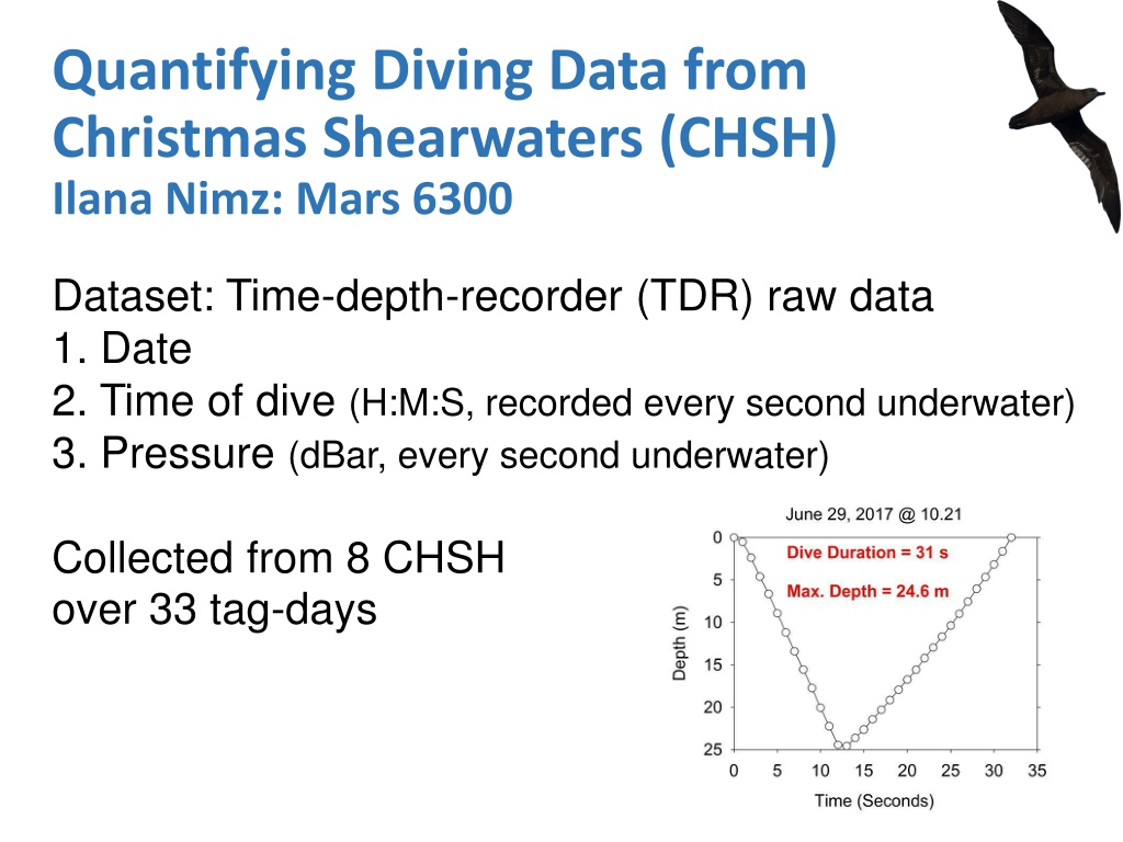
1. Quantifying Diving Data from Christmas Shearwaters (CHSH) Ilana Nimz: Mars 6300 Dataset: Time-depth-recorder (TDR) raw data 1. Date 2. Time of dive (H:M:S, recorded every second underwater) 3. Pressure (dBar, every second underwater) Collected from 8 CHSH over 33 tag-days

2. Objective: Quantify Diving of Christmas Shearwaters (CHSH) Hypothesis: CHSH are diving exclusively during daylight hours (civil twilight a.m. to civil twilight p.m.) Prediction: CHSH dive more frequently in the late afternoon and evening, prior to civil twilight Approach: Summarize dive profiles from TDR raw data Standardize time across 3 months of tagging (Jun-Aug) by dividing 24hrs into 4 time blocks 1) Twilight + 3.5 hrs, 2) Middle of Day, 3) Twilight -3.5 hrs, 4) Night Start by exploring correlations between depth measurements and dive frequency via ordination

3. Dataset Description Main_CHSHsummary.wk1 (main matrix) Dives per Hour: # dives/time-block hrs Maximum Depth: meters Average Maximum Depth: meters Median Maximum Depth: meters %CV Max Depth: meters Samples: Bird-Tag Day- Time Block Grouping Variables: Time: Morning 1, Daytime 2, Evening 3, Twilight 4 Bird:Bird # (1-8) 125 samples & 5 variables Samples: Bird-Tag Day-Time Block (Twilight, Morning, Daytime, Evening) Variables: Second_CHSHgroups.wk1 (Second matrix)

4. Dataset Processing Outliers: No outliers given cutoff of 2.0 SD from the grand mean Empty samples: 500 cells in main matrix; % empty = 32 Samples discarded: All night samples were empty- 26 discarded Some morning samples empty- 12 discarded Data transformations / relativizations: -Attempted to normalize w/ log transform- skew and kurtosis reduced but not normal range for all variables, so Non-parametric route! - Using Median to describe non-parametric data: removed average depth column -Give variables the same weight General Relativization (will relativize during ordination) Describe your sample size: Sample total= 85: 19 Morning, 33 Mid-day, 33 Evening

5. Dataset Exploration Dataset Exploration Identifying correlations: Dives/hr and Depth metrics 0.60 0.43 0.60 Weaker correlation with dives/hr and Depth: Max, Med, CV Tau= 0.605, 0.4271, 0.604 0.70 0.60 Max depth & Median depth Strongest Positive Correlation Tau= 0.6951 0.36 Weakest correlation between Med max and CV Tau = 0.3567 *Data not normal, so used Kendall Tau correlation

6. Dataset Analysis NMS_DiveMaxAvgMedCV_RelSor_999 Ordination of plots in metrics space. 85 plots 4 metrics Settings used in the analysis The following options were selected: ANALYSIS OPTIONS 1. REL.SOREN. = Distance measure 2. 6 = Number of axes (max. = 6) 3. 250 = Maximum number of iterations 4. RANDOM = Starting coordinates (random or from file) 5. 1 = Reduction in dimensionality at each cycle 6. NO PENALTY = Tie handling (Strategy 1 does not penalize ties with unequal ordination distance, while strategy 2 does penalize.) 7. 0.20 = Step length (rate of movement toward minimum stress) 8. USE TIME = Random number seeds (use time vs. user-supplied) 9. 50 = Number of runs with real data 10. 999 = Number of runs with randomized data 11. NO = Autopilot 12. 0.000010 = Stability criterion, standard deviations in stress over last 200 iterations. OUTPUT OPTIONS 14. YES = Write distance matrix? 15. NO = Write starting coordinates? 16. NO = List stress, etc. for each iteration? 17. YES = Plot stress vs. iteration? 18. YES = Plot distance vs. dissimilarity? 19. YES = Write final configuration? 20. UNROTATED = Write varimax-rotated, principal axes, or unrotated scores for graph? 21. YES = Write run log? 22. YES = Write weighted-average scores for metrics ? ------------------------------------------------------------------------------ Distance: Rel Sorensen Randomizations: 999 1500 = Seed for random number generator.

7. Results Interpretation 1 significant axis 2.07 = final stress for 1-dimensional solution *Excellent! (lower stress with fewer species ) Minimum stress real data > Minimum randomized stress p-value = 0.024 (23+1 / 999+1) STRESS IN RELATION TO DIMENSIONALITY (Number of Axes) -------------------------------------------------------------------- Stress in real data Stress in randomized data 50 run(s) Monte Carlo test, 999 runs ------------------------- ----------------------------------- Axes Minimum Mean Maximum Minimum Mean Maximum p -------------------------------------------------------------------- 1 2.070 26.608 57.040 0.000 23.970 57.052 0.0240 2 1.145 1.442 1.683 0.000 1.975 40.936 0.2280 3 0.764 0.946 1.296 0.008 1.104 2.161 0.1840 4 0.706 0.834 1.089 0.012 1.030 2.065 0.1320 5 0.645 0.810 1.086 0.039 0.986 1.635 0.1020 6 0.651 0.825 1.166 0.055 0.955 2.308 0.0950 -------------------------------------------------------------------- p = proportion of randomized runs with stress < or = observed stress i.e., p = (1 + no. permutations <= observed)/(1 + no. permutations) Conclusion: a 1-dimensional solution is recommended.

8. Results Interpretation Scree Plot Stress very low at 1st axis- real data High variability of Randomized stress In 1st axis Overlap: 23 times, randomized > real

9. Results Interpretation Coefficient of Determination (% of Variance): Coefficients of determination for the correlations between ordination distances and distances in the original n-dimensional space: R Squared Axis Increment Cumulative 1 .998 .998 Extremely high amount of variance (99.8%) explained with 1 axis Report Orthogonality: N/A- only 1 axis

10. Results Interpretation Strongest correlation indicates Med Max is explaining axis- negative correlation with axis correl_DiveMaxMedCV Pearson and Kendall Correlations with Ordination Axes N= 85 Axis: r dives pe .351 max dep .082 median m -.402 %CV .768 1 r-sq .123 .007 .161 .590 tau .019 -.390 -.525 .328 Most significant correlation with axis: Median Depth Max & Median Max had strong negative influence CV weak positive influence on axis 1 Not much influence from dive frequency

11. Discussion Method What do these results mean for the hypotheses / predictions you proposed ? -Accept hypothesis: CHSH dive exclusively during the day Need further analysis to test predictions, but NMS was good exploration of patterns prior to testing temporal frequency and depth with a grouping test -Max depth and Median Max depth strongest influences -Frequency of dives not as strong as depth measures in axis

12. Discussion Next Steps What do you propose to do for your re-analysis? MRPP- test the prediction to identify when during daylight hours CHSH are diving more frequently What would be the next steps for this study? Look at time under water and time between dives Compare to other shearwater species