The Essentials of International Comparisons: Lecture Highlights

Delve into the intricacies of conducting international comparisons with a focus on country selection, strengths, limitations, hypothesis testing, and more. Explore various methods like multi-level modeling and grasp the significance of senate weights. Gain hands-on experience with cross-national comparisons using real data. Understand the decision-making process behind selecting countries for analysis based on research questions and theoretical arguments.
- International comparisons
- Country selection
- Hypothesis testing
- Cross-national analysis
- Research methodology

Download Presentation

Please find below an Image/Link to download the presentation.
The content on the website is provided AS IS for your information and personal use only. It may not be sold, licensed, or shared on other websites without obtaining consent from the author. Download presentation by click this link. If you encounter any issues during the download, it is possible that the publisher has removed the file from their server.
E N D
Presentation Transcript
Nuts and bolts of conducting international comparisons Lecture 3
Aims 1. To develop thinking of which countries to include in the analysis. 2. To understand the strengths and limitations of different ways of comparing different countries (e.g. multi-level modelling versus separate country estimates) 3. How to conduct two-sample t-tests to test for significant differences between countries 4. To understand corrections for multiple hypothesis testing and whether these should be applied 5. To understand what senate weights are, how they can be calculated, and when they might be needed. 6. Gain experience of conducting basic cross-national comparisons using the TALIS 2013 dataset.
Which countries should I include?
Often one of the hardest things to decide! Things I have done (or seen done): - Compare every country with data available (e.g. PISA rankings). - Compare within a well-defined group of countries (e.g. OECD or EU). - Language spoken (e.g. English speaking; Finland vs Estonia) - Compare against top performers (e.g. Micklewright et al 2014) - Self-selection based upon some factor of interest - Selection because data available (e.g. Jerrim, Vignoles and Finnie 2012) Often no right or wrong (or clear-cut) answer. Judgement call!! My advice always link it back to your research question .. .. Following slides offer some advice / guidance
Question type and country selection Question type: Generalisability - Example = Girls out-performing boys in reading - Which countries do you hypothesise this will hold in? - Every country in the world? Then include every country with data available - Developed countries only? Then include only OECD countries - Only countries with sufficient female rights? Then include only those countries which meet some objective criteria (e.g. http://www.theguardian.com/news/datablog/2013/oct/25/world-gender-gap-index- 2013-countries-compare-iceland-uk) Key point: Becomes harder for people to argue with your choice if it is explicitly linked to your hypothesis / theoretical argument.
Question type and country selection Question type: Impact of institutional structures - Example = Impact of between school tracking and equality in pupil achievement - Countries = Relevant sample size - Sample size is never going to be large. But want to maximise! - Include all countries with relevant data available. - What is the minimum # of countries you need to reasonably answer this question? N 20 in Hanushek and W mann (citations = 620!) Is a sample size of 20 really enough? My opinion Small sample size (# of countries) is why cross-national comparisons will always be limited in answering institutional structure questions.
Question type and country selection Question type: Macro forces - Example = Association between income inequality and social mobility - Countries = Relevant sample size - Want to maximise sample size .. but also want to base on theory. - Should only include countries where link between income inequality and social mobility will (theoretically) hold. - Has been argued in literature that former communist countries should be excluded: - See Andrews and Leigh (2008) - Lots of political / social change when growing up - Income inequality data of low quality - Reasonable arguments put forward. Does this choice make a difference?
The Great Gatsby Curve. .6 .6 US US Jerrim and MacMillian (2014) SK PL A good example of where country selection was difficult .. GB GB .4 .4 Total effect (beta) Total effect (beta) JP JP FR KR FR KR IE IE ES ES IT IT CZ AU AU EE DE DE CA CA DK DK .2 .and this choice makes a big difference to the result! RU .2 AT AT FI FI SE NL BE SE NL BE NO NO 0 0 .2 .3 .4 .2 .3 .4 Gini (LIS average) Gini (LIS average) Correlation 0.85 N = 18 Correlation 0.40 N = 23
Question type and country selection Question type: Benchmarking - Example = How does the SES gap in achievement compare in UK to other countries? - Key point Who do you want to benchmark the UK against? - Probably not. Do I care about UK compares in this respect against Malawi? Every country in the world? - Possibly (given benchmarking exercise). But some (e.g. Australia, US, Canada) likely to be more relevant comparators than others (e.g. Estonia, Chile, Mexico). Other rich countries? - Ok. But this then really starts to move away from a benchmarking exercise Countries of particular interest?
Benchmarking: SES gap in UK in comparative perspective Source: Jerrim (2012) Benchmark England against 23 OECD countries .but then also highlight comparison with five countries of particular interest.
How do I compare estimates across countries?
Two common approaches: Multi-level model Approach 1 Estimate a multi-level (random effects model) Pupil = level 1; School = level 2; country level 3 Very popular to cross-national comparisons in sociology E.g. ESR published 340 papers 2005-2012. 43 (13%) used MLM Data for all countries has to be pooled together into a single datafile. Typically attempting to identify macro-effects (e.g. income inequality) or of institutional structures (e.g. between school tracking)
Two common approaches: Separate country estimates Approach 2 Analyse each country one-by-one Data for each country may be in a separate datafile for each Popular in economics (and education?) Approach (implicitly) advocated by the OECD for PISA Similar to estimating model using pooled data from all countries and including country fixed effects The approach I have used in almost all my papers using PISA / TIMSS .. See PISA 2003 User Guide for further information
I have never used approach 1 Why? Issue 1: Are the countries included in your analysis really a random sample from a population? (Can you really generalise your results outside your sample of countries)? Issue 2: Do you really have enough countries to produce reliable estimates at the country level? - See Bryan and Jenkins (2013) for discussion - Problems even when C 25. (More than many people use) Issue 3: It never feels very upfront regarding the sample size often of most interest - Remember, often interested in country factors so sample size is small! Issue 4: It becomes very tempting to start over-fitting the data! - E.g. including lots of country-level factors (when sample size is so small!)
How to execute approach 2 Example: Comparing SES gap in academic achievement across countries Estimate model of interest separately within each country. ? = ? + ?.??? + ? ?? Parameter of interest is ? the strength of the association between socio-economic status (SES) and children s test scores. Respondent and replicate weights need to be applied to get correct estimates! Will result in a separate estimate of ? and associated SE for each country. Can use these to construct confidence intervals. Will often see results graphed, along with 95% confidence interval as follows ..
Hypothetical example of results Bar = Estimated association between SES in pupil achievement Country C Line = Estimated 95% confidence interval Country B Question Can we tell from this graph which countries are significantly different from one another at the 5 percent level? Country A Is Country A sig diff to Country B? Is Country A sig diff to Country C? 0 20 40 60 80 100 120 Is Country B sig diff to Country C? Socio-economic gap in test scores
Answer.. Country A versus Country B CI for country A overlaps with the point estimate for country B. Can therefore be sure that one can not reject null hypothesis of no difference between country A and country B at the five percent level. Country A versus Country C CI for country A does not overlap with the CI for country C. Can therefore be certain that one can reject null hypothesis of no difference between country A and country C at the five percent level. Country B versus Country C CI for country B overlaps with CI for country C .. .BUT neither CI overlaps the other country s point estimate We can not tell whether difference between country B and country C is statistically significant at the five percent level from this graph.
Two-sample t-test In the situation of country B versus country C, a formal test for statistical significance is required. This is the two-sample t-test defined as: ?? ?? ? ???? = 2+ ???2 2.???(??,??) ??? Where: ?? = Estimated socio-economic gap in country k ??? = Standard error of estimate in country k 2.???(??,??) = The covariance between estimates for countries j and k
Two-sample t-test Note, however, that samples are usually drawn independently across countries This means we can reasonably assume that 2.???(??,??) = 0. Thus, when comparing estimates across countries, the formula reduces to: ?? ?? ? ???? = 2+ ???2 ??? The resulting T-Stat is then compared to the critical value . If it is greater than the critical value, then we can declare that there is a statistically significant difference between countries B and C at the 5 percent level. Recall: Critical value depends upon DF. DF = Number of replicate weights 1 E.g. DF in TALIS = 79; Critical value = 1.9842
Task: Use figures below to formally test for a significant difference between each of the countries SES Gap ( ) SE Country A 50 16 Country B 80 7 Country C 100 7 Note When reaching your conclusion, assume that the critical value is 1.984.
Answers T-statistic for difference Country A Country B Country C Country A - - - Country B -1.72 - - Country C -2.86* 2.02* - No significant difference between country A and B (possible to tell this from CI s alone) Significant difference between country A and C (possible to tell this from CI s alone) Significant difference between country B and C (needed formal t-test)
The problem Typically, we do not compare our country of interest (e.g. the UK) against just other country of interest (e.g. France). Rather, our country is compared to many other countries (e.g. around 60 in PISA). However, the more countries we draw comparisons to, the greater the probability that we will find a difference with respect to at least one other country simply by chance. We should thus not be too confident that this significant difference is real . If you look hard enough you will find something! Something important to take into account when comparing across multiple countries . Choice Whether this issue is recognised implicitly or explicitly
Example of problem Two country comparison We compare the SES gap in UK to France. and test for significance at the 5% level. The real difference in the population is 0 (SES gap equal across the two). Only 5 percent chance that we will incorrectly reject null hypothesis (declare that there is a difference between UK and France when there is not). Multi-country comparison We compare the SES gap in UK to 100 other countries. The real difference is 0 (SES gap equal across all countries) But, as performing 100 tests, your likely to conclude UK sig diff for 5 other countries purely by chance! 99.5% chance you will make at least one incorrect rejection!
Bonferroni corrections. You can recognise this problem either explicitly or implicitly . Explicit corrections Adjust the level where you declare statistical significance. Very common to see in fields like genetics (due to increasing of use of GWAS) ? Bonferroni correction = ?????? ?? ????? ????????? Example Comparing UK to France at 5% level ?????=? 1 = 0.05 1= 0.05 100 = 0.05 ? Comparing UK to 100 other countries ?????= 100= 0.0005
Exercise Using the T-statistics you calculated previously: Convert these into p-values using the following link: http://www.socscistatistics.com/pvalues/tdistribution.aspx Calculate the bonferroni corrected 5 percent significance level For which countries do you now find there to be a significant difference? Have your conclusions regarding significant differences changed now that a correction for multi-hypothesis testing has been made?
Answers P-value for difference Country A Country B Country C Country A - - - Country B 0.0886 - - Country C 0.0052 0.0461 - ?????=? 3 = 0.05 3= 0.0167 No significant difference between country A and B Significant difference between country A and C No Significant difference between country B and C (CHANGED FROM BEFORE)
Issues Widely recognised Bonferroni correction goes too far the other way . Too conservative! Reduces chance of making a Type I error (Incorrect rejection of null) .. .by increasing the chance of a Type II error (Incorrectly not rejecting the null) Alternatives have been proposed Benjamini and Hochberg correction http://nebc.nerc.ac.uk/courses/GeneSpring/GS_Mar2006/Multiple%20testing%20corrections.pdf Less conservative, but a little more complex to implement. Conclusion Important issue to recognise / understand in cross-country comparisons . whether you make this explicit (via a correction) = judgement call!
Use of multiple corrections in PISA OECD policy on whether to make Bonferroni correction when declaring statistical significance in their rankings seems to have changed over time .. 2000 results Presented results with Bonferroni correction 2003 results Presented results both with and without Bonferroni correction applied 2006 onwards No Bonferroni correction made Reason given: A lot more countries took part in 2006 than 2000. Adjusted p-value would fall from 0.0017 (2000) to 0.00009 (2006) Considered prohibitively strict Implication Different critical values have been applied across cycles Some differences declared as NS in 2003 would have been declared as SIG in 2006
International total and averages The OECD reports contain two statistics that, at face value, seem quite similar: OECD total (aka house average ) OECD average (aka senate average ) But they contain different results! What is the difference between them? How do we calculate them? When is it appropriate to prefer one over the other? Source: PISA 2012 report
International average Very straightforward to understand Say you have PISA scores for 30 countries. Then the international average across these 30 countries is simply: ?=30???? ?????? ?=1 ?????? ?? ????????? In other words, simply take the mean of the statistics that have been produced separately for each country. Key point: Gives each country equal weight when calculating international statistics (such as the OECD average)
Senate weights Senate weights often provided in international databases for ease of calculation These weights basically re-scale the final respondent weight (e.g. student weight in PISA) .so that the sum of these weights then equals the same value (e.g. 1,000) for each country. If you then have all countries included within one datafile .. .you can apply this senate weight (rather than the final student weight) to easily calculated the international average (and other international statistics) A note of caution If you make sample selections (e.g. drop immigrants from your analysis) senate weights provided unlikely to continue to equal same constant in all countries I.E. They will not longer weight each country in your analysis equally! .so you will need to adjust them
International total / House average Also known as the house average Pool all of your countries of interest into a single datafile Estimate your statistic of interest using this pooled datafile, applying the final respondent weight Each country will then be weighted by its population size Large countries will have a much bigger influence upon the figure produced E.g. United States will drive the house average if calculated for North America
Example: % who attend pre-school across 6 countries In this example, choice between house and senate average make a big difference .. Proportion who attended pre-school Country Sample size Population size USA 4,914 3,495,270 98.5 Albania 4,336 38,794 74.6 Why? US is an outlier compared to other countries .. Croatia 4,969 45,172 73.2 Lithuania 4,590 32,847 35.0 Montenegro 4,683 7,608 69.5 Kazakhstan 5,798 208,013 67.2 and has a particularly big weight House average (Population weighted) 94.2 Senate average (Equally weighted) 69.7
Which figure should I prefer / report? Depends upon your question / interest. Example You are interested in private schooling in South America The international ( senate ) average will allow you take make statements like: In the average South American country, X percent of children are enrolled in private school. The international total ( house average ) will allow you take make statements like: X percent of 15 year olds across South America are enrolled in a private sector school. Think Are pupils/teachers or countries your unit of interest?
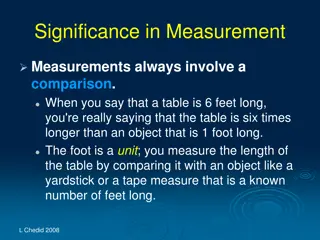
Why standardise? Standardisation (z-scores) very common across social sciences. Aids interpretation E.g. People who know nothing about PISA will not know whether a difference of 50 test points is big or small Concern is in relative rather than absolute differences In many applications, convert pupils test-scores into a z-score metric: ???? ????? ???? ???????? ????????? ??????= Then express results / differences in terms of standard deviations E.g. The rich-poor gap in children s test scores is 0.8 standard deviations in the UK versus 1.1 standard deviations in the United States. Complication in x-national analysis Different ways to standardise ..
National z-scores (standardisation) Standardise variables separately within each country: ???? ????? ???????? ???? ???????? ???????? ????????? ?????????= Example UK: National mean = 490; national SD = 110 Finland: National mean = 520; national SD = 85 Difference mean and SD used in each country Implications Forces distribution of test scores to be similar (mean 0 and SD 1) within each country . Thus abstractsfrom differences in variance / inequality in variable across countries . Focus becomes upon differences in rank position across countries .
International z-scores (standardisation) Standardise variables across all countries together ???? ????? ????????????? ???? ????????????? ???????? ????????? ??????????????= Same mean and SD used to standardise for each country Note possible to use either house or senate international figures .. Implications Distribution of test scores continues to differ across countries (i.e. unequal variances) Thus results continue of incorporate differences in variance / inequality across countries .
Example. Want to estimate the parental education gap in children s test scores: ???? ????? = ? + ?.???????? ????????? + ? Where ? = Difference between children where at least one parent holds a degree versus those where neither parent holds more than high school education ???? ????? can either be standardised nationally (x-axis) or internationally (y-axis) .. How does this choice change results?
Results: National vs International (house) z-scores 1. Effect sizes tend to be bigger when using national z- scores (points fall below 45 degree line). Why? National SD tend to be smaller than international SD Hence smaller value in denominator Leads to bigger effect sizes QUB TAP SVK ISR 1 QUC CHL SGP BEL INTERNATIONAL POL CZE URY 2. Some countries affected more than others Why? Chile has a particularly small national SD Chinese Taipei particularly large national SD BGR HUN TUR PER RUS HRV PRT .75 CAN GRC AUS LUX QRS QCN AUT FRA ARE IRL DEU USA LTU NLD ESP 3. Country comparisons can look quite different depending on which is used E.g. France vs Columbia Both 0.75 national standard deviation difference But falls to 0.50 in Columbia when using international SD Why? National z-score abstracts from the low inequality (SD) in Columbia s PISA test scores SVN VNM NZL QAT BRA ROU THA KOR HKG CRI TUN DNK MYS COL ARG .5 JPN SRB QUA FIN LVA KAZ ISL CHE GBR ITA NOR SWE JOR EST IDN MEX .5 .75 NATIONAL 1
International house vs International senate z-scores QUB TAP SVK ISR 1 QUC CHL SGP BEL POL It makes almost no difference which approach you use when it comes to international standardisation! CZE URY HOUSE BGR HUN PER RUS TUR HRV PRT QRS .75 AUS CAN LUX QCN GRC AUT FRA ARE IRL DEU USA LTU ESP NLD SVN VNM NZL BRA QAT ROU THA KOR HKG CRI TUN COL DNK MYS ARG JPN QUA SRB .5 FIN ISL KAZ CHE GBR IDN MEX JOR LVA EST ITA NOR SWE .5 .75 1 SENATE
Comparing binary outcome models across countries
Example question Outcome of interest may be binary . E.g. SES difference in a young person going to university (0 = No; 1 = Yes) Would be reasonable to investigate how this differs across countries .. Logistic regression would often be used to estimated such binary outcome models .. .with results often presented in terms of odds-ratios or log-odds However, these estimates may not be comparable across countries due to an infrequently discussed methodological issue
The issue See Mood (2010) article in European Sociological Review Logistic regression Way of modelling a binary outcome (y) as the observed outcome of a continuous (though unobserved) latent trait (y*), where: y = 0 y = 1 if y* < T if y* > T Where T is some unknown threshold value. Can write this as a latent variable model: ?? = ? + ?.??+ ?? (1)
The issue To estimate (1), need to assume that ?? follows a particular distribution. Logistic regression Assume follow a logistic distribution with fixed variance = 3.29 Under this assumption, one can estimate as a logit model: ? ?? 1 ?= ? + ?1.?? (2) Where: P = Probability that y = 1 NOTE: latent trait model in (1) formed of both explained and unexplained variance BUT: when we estimate model 2 as a form of this latent trait model, the unexplained component is fixed .
The issue When covariates are added to the logistic regression model, the explained variance has to go somewhere! Can t change the unexplained variance component (as fixed) .. hence increases the variance (and hence the scale) of the dependent variable BUT When the scale of the dependent variable changes, so does our estimate of the parameter of interest (b1) IMPLICATIONS Log-odds / odds-ratios can differ/change across groups (e.g. countries) simply because of differences in unobserved heterogeneity rather than there being a true difference of substantive importance Adding controls that are not associated with the covariate of interest (but is nevertheless associated with dependent variable) influences parameter of interest . {different to situation under OLS}
Implications for x-national comparisons: Example Aim Compare SES gap in HE participation in country A and country B First estimate: ??? = ? + ?.??? ? ? Where: ? = SES gap in log-odds Assume to begin that: - The true SES gap is equal across these countries - Same amount of unobserved heterogeneity in country A and B Therefore Results are comparable across countries. Correctly find that ??= ??
Example Now say we re-estimate the model, but now also controlling for gender ??? = ? + ?.??? + ?.?????? ? ? Assume that: - In both countries gender is unrelated to SES (i.e. it is not a confounder) -Gender strongly associated with HE participation in country A - .but gender not associated with HE participation in country B We find that: ??> ?? (estimated SES gap has increased in country A) ??= ?? (no change in SES gap in country B) Therefore: ??> ??


")
")

 z-scores")