Understanding Sampling Uncertainty: A Comprehensive Overview
Sampling uncertainty arises due to variations in sample values, impacting statistical estimates. Larger samples reduce uncertainty, providing more precise estimates. Adequate sample sizes are crucial, especially for comparing different groups or magnitudes of effects. By quantifying uncertainty, researchers can make more robust inferences and draw reliable conclusions from their studies.

Download Presentation

Please find below an Image/Link to download the presentation.
The content on the website is provided AS IS for your information and personal use only. It may not be sold, licensed, or shared on other websites without obtaining consent from the author. Download presentation by click this link. If you encounter any issues during the download, it is possible that the publisher has removed the file from their server.
E N D
Presentation Transcript
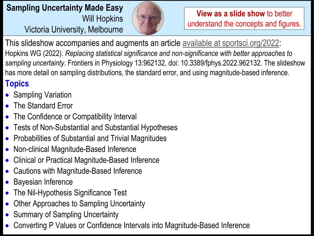
Sampling Uncertainty Made Easy View as a slide show to better understand the concepts and figures. Will Hopkins Victoria University, Melbourne This slideshow accompanies and augments an article available at sportsci.org/2022: Hopkins WG (2022). Replacing statistical significance and non-significance with better approaches to sampling uncertainty. Frontiers in Physiology 13:962132, doi: 10.3389/fphys.2022.962132. The slideshow has more detail on sampling distributions, the standard error, and using magnitude-based inference. Topics Sampling Variation The Standard Error The Confidence or Compatibility Interval Tests of Non-Substantial and Substantial Hypotheses Probabilities of Substantial and Trivial Magnitudes Non-clinical Magnitude-Based Inference Clinical or Practical Magnitude-Based Inference Cautions with Magnitude-Based Inference Bayesian Inference The Nil-Hypothesis Significance Test Other Approaches to Sampling Uncertainty Summary of Sampling Uncertainty Converting P Values or Confidence Intervals into Magnitude-Based Inference
Sampling Variation A sample provides only an approximate estimate of the true value of a simple statistic (e.g., a mean) or an effect statistic (e.g., mean change in performance). Another sample would give a different value of the statistic: that's sampling variation. Therefore there is uncertainty in a sample value: samplinguncertainty. The larger the sample, the less the sampling uncertainty. It is only when samples are huge that different sample values would always be practically the same and therefore be a precise estimate of the true value. By truevalue I mean the huge-samplevalue: the value if you used your sampling method to get a huge sample, and if you used your methods to measure and analyze the huge sample. Your sampling method will always produce a biased sample of a population of interest. Example: you are interested in top-level football players, but a sample from your city or region does not represent the population of top-level players in your country or in the world. A sample would be unbiased if it were chosen randomly from the population of interest. But a random sample of a population is practically unobtainable. So your statistics and their uncertainties apply to a sub-population similar to your sample. Imagine you made a population by duplicating exactly your sample many 1000s of times. That's the kind of population to which your statistics and their uncertainty apply. You should do a study with at least the minimum desirable sample size. This sample size gives acceptable uncertainty (or adequate precision). Depending on the design and statistic, it can be as low as 10, but it is usually much greater.
Sometimes, for logistic or other reasons, you can't avoid a small sample size. But you can't increase your sample size, for example, by adding up the numbers of females and males, because you can't assume that the effect is the same for females and males. So you need a sample size for adequate precision for the effect in males alone, and the same sample size for the females alone. And if you want to compare females and males, you need twice as many males and twice as many females! See the resources on sample-size estimation at Sportscience for more. So, if you have to use a small sample size, use a sample of one kind of subject. It's important to determine the sampling uncertainty in an effect. Incredibly, with just one sample, you can quantify the uncertainty in terms of the spread of values you would expect to see if you did repeat the study many times. Those values would form a probability distribution called the sampling distribution. Values similar to the true value would occur more frequently than values much smaller or larger than the true value. With a large-enough sample size, the sample values have a bell-shape known as the normal (or Gaussian) distribution. "Large enough" depends on the statistic and data, but even really small sample sizes are usually large enough. And for mean effects, it's actually a t distribution (a normal distribution for a finite sample). Proportion (probability) of sample values sampling distribution centered on the true value Sample value true value
Note that the original data are never normally distributed, but an effect statistic is almost always practicallynormally distributed, thanks to the Central Limit Theorem. Amazing! Some researchers waste their time by testing for normality of the original data, then needlessly using so-called non-parametric analyses when they think the data are non-normal. A sample variance (SD2) has a chi-squared distribution, but this is normal for large samples. The normal distribution always has the same bell shape; only the spread differs. The spread of the distribution, and therefore the sampling uncertainty, can be summarized with a standard error (SE) or a confidence (or compatibility) interval (CI). The Standard Error The SE is the standard deviation you would expect to get if you repeated your study many times (with samples of the same size, using the same sampling method and analysis), and calculated the standard deviation of all the sample values of the effect. As such, the SE represents expected typical variation in the statistic from sample to sample. The simplest SE is the SE of the simplest statistic, the mean. SE = SD/ n, where SD is the SD of individual values in the sample, and n is the sample size. If the statistic is a mean change (e.g., in performance resulting from training a sample of n athletes), the SD in this formula is simply the SD of the individual change scores. If the statistic is a difference in means between two groups of individuals (e.g., the difference in the means of females and males, or the difference in mean changes in an experimental and control group), the formula for the SE involves the SDs and sample sizes of each group.
With a normal distribution, the true value 1SD contains ~two-thirds (68%) of the data. So, the true value of the statistic the sample SE contains 68% of sample-statistic values: Proportion of samples sampling distribution centered on the true value Probability of true value sampling distribution centered on the sample value area = 68% area = 68% true value 1SE true value + 1SE sample value 1SE sample value + 1SE Sample value True value true value sample value Rearranging, the sample value SE contains the true value for 68% of sample values. These are so-called frequentist interpretations of the true value, sample value, and SE. You can also say that the normal or t distribution centered on the sample value is a probability distribution for the true value. This is the so-called Bayesian interpretation of the sampling distribution. More on this later! So the sample value minus its SE through to the sample value plus its SE has a 68% chance of including the true value. But people want more "confidence" than 68% about what the true value could be. Hence
The Confidence or Compatibility Interval This is just like the sample value its SE, but you want to be 90%, 95% or even 99% confident about what the true value could be. For example, if you repeated the study with a huge sample size to get the true value, then the 90%CI derived from your original sample has a 90% chance of including the true value. And there is a 10% chance the true value falls outside the 90%CI. The value 1.64 SE is the 90%CI. The value 1.96 SE is the 95%CI. The value 2.58 SE is the 99%CI. Obviously, a wider interval gives more confidence about including the true value. Actually, these multiples of the SE are values of the z statistic, from the normal distribution that you get with huge samples. With smaller samples the sampling distribution of a mean effect is a t distribution, so the multiples are values of the t statistic, which are a bit bigger than z. Examples: for a sample size of 1000, the 90%CI are 1.64 SE (z and t are practically the same) for a sample size of 30, the 90%CI are 1.70 SE for a sample size of 20, the 90%CI are 1.73 SE for a sample size of 10, the 90%CI are 1.83 SE. Probability of true value 90%CI area = 90% area = 5% area = 5% True value sample value These SEs would also get bigger with smaller sample sizes.
The confidence interval, interpreted as what the true effect could be, provides a good simple approach to deciding whether or not there is an effect. This is almost always the main research aim; it's called making an inference about the effect. Given sampling uncertainty, you can never be sure that there is absolutely no effect (e.g., the change in the mean is exactly zero.) So "there is no effect" means the effect is trivial (unimportant, harmless ). And "there is an effect" means the effect is substantial(important, harmful, beneficial ). Hence you need smallest important values for an effect that divide the range of effect magnitudes into substantial negative, trivial, and substantial positive. Then you simply state the magnitude of the lower and upper confidence limits: Value of effect statistic Conclusion: negative ( ive) trivial positive (+ive) the effect is +ive (to +ive) +ive (to +ive) smallest important negative positive trivial to +ive trivial to +ive This is a good method to deal with sampling uncertainty. trivial to +ive trivial (to trivial) ive to trivial ive to trivial ive to trivial ive (to ive) ive to +ive unclear
Improve the interpretation by introducing magnitude thresholds for moderate, large, very large and extremely large. small+ive small ive trivial moderate Conclusion: the effect is small to moderate +ive small (to small) +ive This is a better method to deal with sampling uncertainty. trivial to moderate +ive trivial to small +ive trivial to small +ive trivial (to trivial) small ive to trivial small ive to trivial moderate ive to trivial moderate to small ive small ive to small +ive unclear The thresholds for the various kinds of effect are in the sideshows in the article linked to Linear models & effect magnitudes at sportsci.org. See also the appendix in the article Magnitude-based Decisions as Hypothesis Tests at sportsci.org/2020. Here are thresholds for small, moderate, large, very large and extremely large effects: correlations: 0.10, 0.30, 0.50, 0.70, 0.90 (not for validity or reliability correlations!) standardized differences in means: 0.20, 0.60, 1.20, 2.0, 4.0 (use with caution!) changes in competition performance: 0.30, 0.90, 1.6, 2.5, 4.0 (of within-athlete variability) proportions: 10%, 30%, 50%, 70%, 90% (for Likert scales and match winning/losing) count, risk and hazard ratios: / 0.90, / 0.70, / 0.50, / 0.30, / 0.10 (e.g., for injuries).
Bootstrapping or resampling is a method for generating confidence limits, when you have "difficult" effects for which the usual sampling distribution is not known. Example: a comparison of two correlation coefficients from the same sample. Bootstrapping gives the same confidence limits as those from known sampling distributions. With this method, you make an imaginary population consisting of your sample duplicated infinitely. You then draw randomly a sample of the same size as your original sample from this population. Draw at least 3000 samples in this manner. You actually do it by randomly sampling with replacement from your original sample. The resulting distribution of values is the sampling distribution you want. It's pure magic! The sample size needs to be at least 20 for the method to work properly. The median of the 3000+ values should be the same as the original sample statistic. If it's not, you've done something wrong! And the 5th percentile and the 95th percentile of the 3000+ values are the lower and upper 90% confidence limits. The bootstrapped distribution of values can also be used with the various methods for dealing with sampling uncertainty.
Why "compatibility" interval? The preeminent statistician Sander Greenland prefers this term. In order for the interval to represent confidence in the true (here: population) value, you must assume that the sampling method produces an unbiased sample of the population. But the effects in your sample apply only to a sub-population like your sample. And you must assume that the statistical model that calculates the sample statistic is realistic. Comparisons of means require no assumptions, but "adjusting" for subject characteristics and estimating their effects usually involves an assumption of linear effects, which may be unrealistic. And you must assume that your measurement methods do not introduce systematic errors. In other words, the measurements need to have acceptable high validity. With compatibility, you are supposed to be reminded about these assumptions. Specifically, you are supposed to say to yourself "the range of values represented by the interval are most compatible with my sample data and my model." But now I am not sure how to interpret the level (90%, say) of the compatibility interval. And there is no mention of the true (huge-sample or population) value. So apparently, I can't use this concept to decide whether or not I have an effect. To make such decisions, you have to assume that the CI represents confidence about what the true value could be, and values outside the CI represent what the true value couldn't be. Deal with the assumptions by doing a sensitivity analysis, in which you estimate the effect of realistic worst-case violations of the assumptions on the width and disposition of the CI. The concept of couldn't be or incompatibilitymakes it easy to understand the next method
Tests of Non-Substantial and Substantial Hypotheses If the confidence interval falls entirely in substantial positive values, then the effect couldn't be non-substantial-positive (i.e., it couldn't be trivial or substantial negative). That is, non-substantial-positive values are not compatible with the sample data and model. In other words you reject the non-substantial-positive hypothesis. Therefore you conclude that the effect can only be substantial positive. Here are all such hypotheses you can reject, and the resulting conclusions: Hypothesis the effect is Conclusion: negative trivial positive rejected non +ive non +ive +ive +ive ive only ive only not ive, or trivial to +ive not ive, or trivial to +ive This is an OK method to deal with sampling uncertainty. ive only ive & +ive trivial not ive, or trivial to +ive +ive only +ive only non +ive, or ive to trivial non +ive, or ive to trivial +ive only non +ive, or ive to trivial non ive none ive no conclusion Hypothesis testing is obviously a blunt instrument for making conclusions. It would be nice to distinguish between these two, or these three. See later. Some researchers like hypothesis testing, because it has a well-defined error rate
Keep in mind that nothing is certain about effects. You could be wrong when you reject a non-substantial or non-trivial hypothesis and thereby decide the effect is substantial or trivial. The error rate is at most 5% (the "alpha"), for testing these hypotheses with a 90%CI. There is the same maximum error rate for rejecting a substantial hypothesis via a 90%CI. When you have more than one effect, the chances of being wrong increase. Example: for two decisive independent effects, each with an error rate of 5%, the chance of making at least one error is approximately 5% + 5% = 10% (more precisely, 9.8%.) Hence, if you want to control inflation of error with multiple effects (you don't have to), you could declare only one of these two effects to be decisive. Or you could use a test with a lower alpha (via a CI with a higher level). Example: with a 95%CI, the maximum error rate is 2.5%, so the maximum combined error rate for two effects is 2.5% + 2.5% = 5%. Example: a 99%CI has a maximum error rate of 0.5%, so you can have up to 10 decisive effects based on a 99%CI and keep the error rate below an acceptable 10*0.5 = 5%. The price you pay for using lower alphas (wider CIs) is fewer decisive effects! I always show 90%CI, but I sometimes highlight effects that have adequate precision at the 99% level by showing them in bold in tables, regardless of the number of effects. See the article Magnitude-based Decisions as Hypothesis Tests and the accompanying slideshow at sportsci.org/2020 for a full description of error rates.
You could refine hypothesis testing by using additional hypotheses to allow you to conclude that the effect is decisively small (the CI falls entirely in small values), or decisively at least moderate +ive (the lower confidence limit is moderate), and so on. You could even use a CI with a lower level than 90% (e.g., a 50%CI) to allow you to distinguish between these three otherwise identical conclusions: But it's confusing, unconvincing, and hard to explain in a publication. There is a better way Probabilities of Substantial and Trivial Magnitudes The extent of overlap or non-overlap of a CI with a magnitude can be expressed as the area of the sampling distribution falling in that magnitude. These areas are chances that the true effect has a substantial negative, trivial, and substantial positive value. The areas are calculated from the known or bootstrapped sampling distribution. negative trivial positive 90%CI sampling distribution area = 53% area = 44% area = 3% Value of effect statistic
The chances of substantial and trivial magnitudes can be expressed as numeric and qualitative probabilities. A similar qualitative scale is used by the Intergovernmental Panel on Climate Change to communicate plain-language uncertainty in climate predictions to the public. The probabilities of substantial ive and +ive are actually p values for tests of the hypotheses that the effect is substantially ive and +ive. Example: if the chance of ive is 3%, p = 0.03, so you reject the hypothesis that the effect is ive at the 5% level (p < 0.05). And 1 minus these probabilities are actually the p values for the tests of the hypotheses that the effect is not substantially ive and +ive. Example: if the chance of +ive is 44%, p+ = 0.44, so 1 - p+ = pN+ = 0.56, so you can't reject the hypothesis that the effect is not substantially +ive. But if the chance of +ive is 96%, p+ = 0.96, so 1 - p+ = pN+ = 0.04, so you can reject the hypothesis that the effect is not substantially +ive, i.e., the effect is decisively +ive. It's easier to think about the probabilities for a magnitude than against a magnitude. So if an effect is very likely substantial, it is decisively substantial, in terms of an hypothesis test at the 5% level or in terms of coverage of a 90%CI. Chances <0.5% 0.5-5% 5-25% 25-75% 75-95% 95-99.5% Probability <0.005 0.005-0.05 0.05-0.25 0.25-0.75 0.75-0.95 0.95-0.995 Qualitative most unlikely very unlikely unlikely possibly likely very likely >99.5% >0.995 most likely
The probabilities can also be expressed as level of evidence against or for a magnitude. Chances <0.5% 0.5-5% 5-25% 25-75% 75-95% 95-99.5% Probability <0.005 0.005-0.05 0.05-0.25 0.25-0.75 0.75-0.95 0.95-0.995 Qualitative most unlikely very unlikely unlikely possibly likely very likely Evidence against or for strong against very good against good against (weak for) some or modest for (against) good for (weak against) very good for This is a great method to deal with sampling uncertainty. excellent or strong for >99.5% >0.995 most likely Level of evidence is a welcome alternative to yes-or-no decisions about magnitudes. So there is less concern about error rates and managing inflation of error. And the qualitative terms and evidence terms provide a more nuanced assessment of magnitude for effects like these: Once effects like these are decisively not substantially negative (or positive), then you want to know the evidence that they are trivial or substantially positive (or negative). So you focus on the probabilities and evidence for a magnitude, not the probabilities and evidence against a magnitude. This approach is the basis of
Non-Clinical Magnitude-Based Inference The qualitative magnitude can still be expressed as the lower and upper 90%CLs, but I usually state the observed magnitude. Then you state the qualitative probability that the effect is substantial and/or trivial, when either of these is at least possible and the effect has adequate precision. Conclusion small+ive small ive trivial moderate Conclusion via MBI: the effect is moderate, most likely +ive abbreviated moderate **** small *** small, very likely +ive small ** trivial 0 * small, likely +ive trivial, possibly trivial & +ive This is a great method to deal with sampling uncertainty. likely trivial (& not ive) very/most likely trivial likely trivial (& not +ive) small, possibly ive & trivial trivial 00 trivial 000/0000 trivial 00 small *0 small ** small ***/**** trivial small, likely ive small, very/most likely ive For unclear effects, show observed magnitude without probabilities. trivial, unclear In a table or figure, the probabilities can be abbreviated with asterisks and superscript 0s. These draw more attention to effects with more evidence. Don't worry about trying to show the terms unlikely, very unlikely and most unlikely. But some researchers like to show all three chances. Example: 3.4/53/44 %. OK. Expressed as p values, these are also convenient for those who like to test hypotheses.
In non-clinical MBI, a magnitude is decisive if it is at least very likely. In other words, the 90%CI falls entirely in substantial (or the 95%CI falls entirely in trivial). So it's equivalent to rejecting the hypothesis that the effect does not have that magnitude. And the error rates are the same as for testing substantial and non-substantial hypotheses. As with hypothesis testing, the chances of making at least one mistake increase, when you have more than one effect. Example: If the chances of being substantial for two effects are 96% and 97% (both very likely), you would like to conclude that both are decisively substantial. But the chances that each is not substantial are 4% and 3%. If the effects are independent of each other, the chance that at least one of them is not substantial is 4% + 3% = 7%, which is greater than the 5% error threshold for either effect. Hence, if you want to control inflation of error (you don't have to), you could declare only one of these two effects to be decisively substantial. Or you could set a higher probability threshold for deciding that an effect is decisive. As before, making decisions with a 95%CI would mean a maximum error rate of 2.5%, and a magnitude would need a 97.5% chance to be decisive. So the maximum combined error rate for two effects would be 2.5% + 2.5% = 5%. Unfortunately, in this example, neither effect would be decisive with a 95%CI. As before, using a higher level for the CI is the usual way to control inflation of error. So with lots of effects, you pay more attention to those that are most likely, and to those highlighted in bold (adequate precision at the 99% level). But don't ignore magnitudes with adequate precision at the 90% level.
Clinical or Practical Magnitude-Based Inference This is the version of MBI to use when substantial means beneficial or harmful. The effects of implementable treatments or strategies are evaluated with this approach. You would implement an effect that could be beneficial, provided it had a low risk of harm. I chose "could be beneficial" to mean possibly beneficial, or >25% chance of benefit. I chose "low risk of harm" to mean most unlikely harmful, or <0.5% risk of harm. An effect with >25% chance of benefit and >0.5% risk of harm is unclear (has inadequate precision): you would like to use it, but you dare not. An unclear effect is equivalent to a 50%CI overlapping benefit and a 99%CI overlapping harm. But don't show this asymmetrical CI. Instead, keep showing a 90%CI. The different probability thresholds or CIs for benefit and harm are equivalent to placing more importance on avoiding harm than on missing out on benefit. Effects that are at least possibly beneficial and are highlighted in bold (adequate precision at the 99% level) are most unlikely harmful and are therefore implementable. In a less conservative version of clinical MBI, an otherwise clinically unclear effect is considered implementable when the chance of benefit far outweighs the risk of harm (odds ratio of benefit/harm >66; the 66 is the odds ratio for borderline benefit and harm). But consider controlling the inflation of the risk of harm with several implementable effects. Before implementing, consider: sample and model assumptions; rewards of benefit; costs of harm; and the chances, rewards and costs of any beneficial and harmful side effects.
Cautions with MBI Unclearis a good word to describe an effect with inadequate precision, but If the main effect in a study is unclear, you can, if you wish, state the magnitude (small, moderate ) of its lower ( ive or reduction) and upper (+ive or increase) confidence limits. And of course, state that the study needs to be repeated with a bigger sample size. Avoid using clear effect. Instead, use adequate precision. Use clear, clearly or decisively only when a magnitude is very likely or most likely. So, if an effect is possibly or likely substantial (or trivial), do not end up carelessly concluding that there is (or isn't) an effect. Instead, keep possibly or likely in the conclusion, or conclude that there is some evidence or good evidence that the effect is substantial (or trivial). Be extra careful when you use small, moderate, etc. to describe the observed effect and probabilities to describe the true effect. Example: observed large and very likely substantial is different from very likely large. It's very likely large only if there is at least a 95% chance it is large. Otherwise it is only possibly or likely large. An effect can be unclear with clinical MBI but have adequate precision with non-clinical MBI, and vice versa. Don't cheat here. If you are doing the study for evidence that a treatment or strategy could be beneficial or harmful, you should use clinical MBI. Effects of modifiers usually require non-clinical MBI. Example: a positive effect of gender on performance would not usually lead to a recommendation to change gender!
Bayesian Inference As with MBI, you estimate chances of the magnitudes of the true effect. Here you include prior belief or prior information about the probability distribution of the true effect with your data to get a posterior distribution, from which you get the chances: Prior distribution + your data posterior distribution. In a full Bayesian analysis, a prior distribution is needed for every parameter in the statistical model. This gets really complicated, and it's hard to justify your beliefs in the priors or difficult to derive relevant prior distributions from publications. In a simplified approach promoted by Sander Greenland, all you need is a single prior representing your prior uncertainty in the effect for chosen values of effect modifiers in the statistical model. For example, if you had males and females in a study, and you estimated the effect for males, then you would use a single prior representing your prior uncertainty in the effect for males. This approach is easily implemented with a spreadsheet. You input the prior and your data as confidence intervals; the spreadsheet gives you the posterior confidence interval and probabilities that the true effect is substantial and trivial. Greenland's approach to Bayesian analysis is useful to prove that MBI is Bayesian. Make the prior CI so wide that it is non-informative. The posterior CI is then identical to the original CI derived from your data.
Hence the original CI represents uncertainty in the true effect, when you opt for no prior information. That's MBI: MBI is Bayesian inference with a non-informative prior. I do not recommend Bayesian inference with an informative prior. An informative prior based on belief is difficult to justify and quantify. The more informative it is, the more likely it is to bias the effect towards what you think it could be or what you would like it to be. A meta-analysis can provide an objective informative prior, but a published meta-analysis may not provide enough information about the effect for your subjects in your setting. You could do a meta-analysis yourself to generate the prior. But it's more sensible to do your study first, without a prior, then do a meta-analysis that includes your study, because... People are more interested in the effects in a meta-analysis than in the effect in your setting. If your sample size is really small, the magnitude of the lower and/or upper CL of the effect, or even the observed magnitude, may be unrealistically large. In that case, a weakly informative prior will "shrink" the estimates to something more realistic. But is it worth it? I don't think so. I think it's better to show the really wide CI, to remind yourself and the reader that your sample size was too small. But it's up to you!
The Nil-Hypothesis Significance Test In the NHST approach, you use a p value to decide whether an effect is statistically significant or statistically non-significant. The "nil" refers to no effect: a mean difference of 0, a correlation of 0, or a ratio effect of 1. It's sometimes called the null-hypothesis significance test, but that term can be used for substantial and non-substantial hypotheses. Nil is more appropriate, because you test the hypothesis that the effect is exactly nil. It's easiest to understand significance and non-significance by thinking about the compatibility interpretation of a confidence interval. If the CI does not contain the nil, the nil is not compatible with the sample data and model. In other words, you reject the nil hypothesis, and you say the effect is significant. If the CI does contain the nil, the nil is compatible with the sample data and model. In other words, you fail to reject the nil hypothesis, and you say the effect is non-significant. The CI for NHST is usually a 95%CI. This effect would be statistically significant at the 5% level: And this effect would be statistically non-significant (or not statistically significant) at the 5% level: Some naive researchers refer to an effect like this, which is nearly significant (e.g., p = 0.07), as a "trend"! 95%CI 95%CI 0 Effect values
The NHSTp value is a bit harder to understand. If the nil-hypothesis (H0) is true, the p value is the probability of getting effects as large as your observed effect, or larger, +ive or ive. If the probability is low enough, it means values like yours (or larger) are too unlikely for the nil hypothesis to be true. So you reject the nil hypothesis. In this example, the p value is 0.04 + 0.04 = 0.08, which is >0.05, so the effect is not significant. The correct conclusion about a significant effect is that the effect is greater than zero. And the correct conclusion about a non-significant effect is that the effect could be zero. But researchers mostly interpret significant as substantial and non-significant as trivial. This is the conventional approach to interpreting NHST. In conservative NHST, researchers interpret the magnitude of significant effects, and they interpret non-significant as indecisive. Either way, if you accept that a 90%CI provides decisive evidence for substantial and trivial, it's easy to show that you make too many mistakes with NHST. It all depends on the smallest important effect and the width of the CI. Use one or more of the other methods to make conclusions about magnitudes of effects. Use a spreadsheet at Sportscience to convert an NHST p value into a meaningful conclusion. Probability of sample value sampling distribution centered on the nil hypothesis, H0 p = 0.04 p = 0.04 H0 0 Sample values sample value (opposite sign) sample value (observed)
Other Approaches to Sampling Uncertainty Superiority, inferiority and minimum-effects testing are simply testing of non- substantial hypotheses. Equivalence testing is simply testing of substantial hypotheses. I do not recommend any of the following S values are an alternative way to present low p values, promoted by Sander Greenland. The S value is the number of consecutive head tosses of a coin that would occur with that low probability. Mathematically, the number of tosses is -log2(p). Examples: If p = 0.05, S = -log2(0.05) = 4.3 tosses. If p = 0.03, S = -log2(0.03) = 5.1 tosses. Is it easier for people to think about low probabilities in this way? I don't think so. Very unlikely, less than 5%, or less than 1 time in 20 seem to me to be more understandable. And it's focusing on probabilities against something (rejecting an hypothesis), but we're more interested in probabilities and therefore evidence for something. Second-generation p values appear to be similar to the probabilities of substantial and trivial values, but they can be difficult and misleading to interpret. Evidential statistics is an approach for choosing between two statistical models using the ratio of the likelihoods representing goodness-of-fit. That's OK, but mostly you do not need a quantitative approach to choosing between models. Advocates of this approach then use a likelihood ratio to choose between two hypotheses. That's similar to the odds-ratio approach of clinical MBI, but otherwise you gain nothing by comparing the chances of substantial and trivial magnitudes.
Summary of Sampling Uncertainty Estimate the minimum desirable sample size for one kind of subject, and try to get a sample at least that large. State and justify the smallest and other important values (moderate, large...) for each effect statistic. If you have several effects with the same dependent variable, figures like these help you and the reader make the right conclusions. In text and tables, show the numerical observed effect and confidence limits or confidence interval. Then show the magnitude of the lower and upper CLs for effects with adequate precision; e.g., trivial-moderate. Or show the observed magnitude, with probability of substantial and/or trivial true effect for those with adequate precision; e.g., moderate ****, trivial 0 *, trivial 00, small *0. Show adequate precision at the 99% level in bold, regardless of the number of effects. Do a sensitivity analysis: the effect on the CLs of worst-case violations of assumptions. Describe the level of evidence for a magnitude: weak, some, good, very good, strong. Avoid NHST. If a journal insists on hypothesis testing, explain in your Methods section the equivalence of the above methods with testing substantial and non-substantial hypotheses. See how in Magnitude-based Decisions as Hypothesis Tests at sportsci.org/2020.
The following two slides introduce two relevant Sportscience spreadsheets. Converting P Values into Magnitude-Based Inferences Statistical significance is on the way out, but the associated classic p values will be around for years to come. The NHST p value alone does not provide enough information about the uncertainty in the true magnitude of the effect. To get the uncertainty expressed as confidence limits or confidence interval, you need also the sample value of the effect. Put the p value and sample value into the spreadsheet Convert p values to MBI. The upper and lower limits of the confidence interval tell you how big or small the true effect could be, numerically. But are those limits important? To answer that, you need to know the smallest important value of the effect. You can then see whether the confidence limits are important and thereby decide how important the effect could be. That s OK for non-clinical effects, but if the effect represents a treatment or strategy that could be beneficial or harmful, you have to be really careful about avoiding harm. For such clinical effects, it s better to work out the chances of harm and benefit before you make a decision about using the effect. Even for non-clinical effects, it s important to know the chances that the effect is substantial (and trivial).
The spreadsheet works out the chances and makes non-clinical and clinical decisions from the p value, the sample value of the effect, and the smallest important effect. Deciding on the smallest important is not easy. See other resources at Sportscience. If there is too much uncertainty, the spreadsheet states that the effect is unclear. More data or a better analysis are needed to reduce the uncertainty. Converting Confidence Intervals into Magnitude-Based Inferences Some authors no longer provide NHST p values, or they may provide only an unusable p- value inequality: p>0.05. If they provide p<0.05, you can do MBI approximately by assuming p=0.05. But if they provide confidence intervals or limits, you can do MBI exactly. Once again you need the smallest important value of the effect. You could use the previous spreadsheet, by trying different p values to "home in" on the same confidence limits. Or the spreadsheet designed to Combine/compare effects can be used to derive the magnitude-based inference for a single effect. A spreadsheet in this workbook also does a Bayesian analysis with an informative prior. You have to provide prior information/belief about the effect as a value and confidence limits. The spreadsheet shows that realistic weakly informative priors produce a posterior confidence interval that is practically the same as the original interval, for effects with the kind of CI you get with the usual small samples in sport research. Read the article on the Bayesian analysis link for more.