Estimation of Causal Effects using Propensity Score Weighting

Understanding causal effects through methods like propensity score weighting is crucial in institutional research. This approach helps in estimating the impact of various interventions, such as a writing program, by distinguishing causation from correlation. The use of propensity score matching aids in mimicking random assignment to evaluate the causal effects accurately and address selection bias issues. By exploring examples and limitations, researchers can enhance their understanding of estimating causal effects in research studies.

Download Presentation

Please find below an Image/Link to download the presentation.
The content on the website is provided AS IS for your information and personal use only. It may not be sold, licensed, or shared on other websites without obtaining consent from the author. Download presentation by click this link. If you encounter any issues during the download, it is possible that the publisher has removed the file from their server.
E N D
Presentation Transcript
Estimation of Causal Effects using Propensity Score Weighting in Institutional Research Ling Ning & Mayte Frias Senior Research Associates Neil Huefner Associate Director Timo Rico Executive Director
Outline Understanding causal effects Methods for estimating causal effects Overview of Propensity Scoring methods Example: Estimating the causal impact of a writing program Limitations and conclusion
Causation versus Correlation We are interested in causal effects, not association or correlation. Casual effect describes how an outcome changes (e.g., retention, time to degree, term/cumulative GPA) as a direct result of some treatment (e.g., participation in student support services or academic development programs).
Example: How can we estimate the causal effect of a writing tutoring program? 4.0 when participating Cumulative GPA Causal Effect False Effect FALSE when NOT participating 0.0 Before Participation After Participation Fundamental problem for causal effect: We only observe ONE of the two potential outcomes
Random Assignment Estimating Causal Effect Control Group Treatment Group Gold standard for estimating causal effects: Randomization (if true) creates groups being compared balanced on baseline characteristics Treatment assignment is unrelated to potential outcomes (Unconfoundedness assumption satisfied)
Selection Bias When selection bias occurs, the characteristics of participants do not match those of non participants. STEM (%) participants non participants URM (%) Low Income (%) First Generation (%) Apcredit (mean) SAT Total (mean/100) high school GPA (mean) 0 10 20 30 40 50 60 70
Propensity Score Matching Estimating Causal Effect Propensity Score Matching Mimic Random Assignment Treatment Outcomes Low-income First Generation SAT Score URM Ethnicity Motivation Confidence Participants (Treatment) Selection Bias? Effect Non-Participants (Non-Treatment) Non-Treatment Outcomes
What is PS PS Estimation Logistic regression Estimating the conditional probability of assignment to treatment group given observed covariates k p = = = = = = = = = = + + W ( logit | 1 ) log X x x 0 i i i i i 1 p 1 i where k is the number of covariates; w denotes the binary treatment conditions Main applications of propensity scores*: Matching Stratification Regression adjustment Weighting * Thoemmes, F. J., & Kim, E. S. (2011). A systematic review of propensity score methods in the social sciences. Multivariate Behavioral Research, 46(1), 90-118.
Machine Learning Methods PS Estimation Machine learning methods are state of the art techniques for propensity score analysis that allow researchers to: Readily include many covariates Easier to incorporate multiple different types of covariates in analyses (e.g., binary, ordinal, continuous, skewed variables). Inspect all possible power and interaction terms Avoid issues of model misspecification Easily handle missing data
Machine Learning Methods PS Estimation Benefits to the outcome analysis: Better balance between treatment and comparison group on pretreatment covariates Reduce bias in treatment effect estimates Produce more stable propensity score weights and thus improve precision The Generalized Boosted Model (GBM) is one such machine learning method. TWANG* (Toolkit for Weighting and Analysis of Nonequivalent Groups) * Ridgeway, G., McCaffrey, D., Morral, A., Burgette, L., & Griffin, B. A. (2015). Toolkit for Weighting and Analysis of Nonequivalent Groups: A tutorial for the twang package. R vignette. RAND.
Example: Evaluating the causal impact of a campus-wide writing tutoring program What impact does participation in the Writing Tutoring Program have on students cumulative GPA, retention, and unit progress? Participants 700 students in 2015 freshmen cohort Longitudinal, observational data Non-Participants 3189 students in 2015 freshmen cohort Longitudinal, observational data
Selection Bias Selection bias occurs when the participants in the writing tutoring program compared with non participants differ. STEM (%) participants non participants URM (%) Low Income (%) First Generation (%) Apcredit (mean) SAT Total (mean/100) high school GPA (mean) 0 10 20 30 40 50 60 70
Pretreatment covariates PS Estimation High school academic performance (e.g., high school a-g courses, high school honor courses, units of advanced placement courses taken, units of advanced placement courses completed, ACT test scores/SAT test scores, high school transferred units, high school GPA); High school background (e.g., last high school type, location); Social economic status (e.g., URM, low-income, first generation, parents education, parents income, and family size); Individual characteristics (e.g., sex, age, ethnicity, residential status, international); Major characteristics (e.g., major, STEM). A total of 41 variables were used in generating propensity score.
R code example for generating PS weighting Install.packages( twang ) library(twang) ps.write_tutoring<- ps(group ~ lstype + atog + atoga + atogb + atogc + atogd + atoge +atogf +atogg +hon10+hon11+hon12+eth_1 + urm+ sex+ incomep+ famsizep+ edfather+ edmother+satrt + satrm + satrw + satrr + eop+ gpa+xhrs+ lowincome1+fg+lang+sats1+sats2+actcon+acte+actm+actr+acts+actw+aptaken+ap passed+ + uccorescore+testindex+ schindex+ countypr+ res+ major, data = write_tutoring, estimand = "ATT", stop.method = c("es.mean", "ks.mean","es.max","ks.max"), n.trees = 60000) Source: Ridgeway, G., McCaffrey, D., Morral, A., Burgette, L., & Griffin, B. A. (2016). Toolkit for Weighting and Analysis of Nonequivalent Groups: A tutorial for the twang package. R vignette. RAND.
Diagnostic check for balance 2 participants Non-participants
Magnitude of group differences pre and post PS weighting Group Difference Effect Sizes among Participants and Non-Participants for select baseline covariates before and after propensity score weighting Unweighted Propensity Score Weighted Some Covariates Participants Participants Non-Participants Non-Participants M SD M SD Effect Size M SD M SD Effect Size 0.52 0.5 0.37 0.48 0.31 0.52 0.5 0.49 0.5 0.07 fg(%) 0.4 0.49 0.23 0.42 0.34 0.4 0.49 0.35 0.48 0.11 lowincome (%) 0.59 0.49 0.75 0.43 -0.33 0.59 0.49 0.64 0.48 -0.11 eop(%) 1672.85 262.99 1830 229.23 -0.60 1672.85 262.99 1707.1 257.37 -0.13 satrt 597.65 131.46 625.65 96.37 -0.21 597.65 131.46 608.04 120.07 -0.08 satrm 536.34 94.85 593.25 89.27 -0.60 536.34 94.85 551.53 96.62 -0.16 satrw 509.7 86.27 581.41 88.89 -0.83 509.7 86.27 522.79 91.27 -0.15 satrr 3.93 0.23 4.02 0.23 -0.37 3.93 0.23 3.95 0.24 -0.05 gpa 21.58 14.45 27.96 16.55 -0.44 21.58 14.45 23.14 15.92 -0.11 xhrs 2.78 1.81 3.85 2.2 -0.59 2.78 1.81 3.06 2.01 -0.15 aptaken 2.78 1.81 3.85 2.2 -0.59 2.78 1.81 3.06 2.01 -0.15 appassed 5604.25 366.42 5846.83 355.05 -0.66 5604.25 366.42 5650.8 368.05 -0.13 schindex
GBM PS weight distribution for the comparison group Non-Participants: Before Weighting (N=3189) After Weighting (N=1132) Propensity Weights for Non-Participants
Treatment Effect Analysis Two-level random intercept model estimated using Mplus Estimates of Treatment Effect on Cumulative GPA Weighted Two-level Random Intercept Model confidence interval Estimate S.E. Est./S.E. P-Value Effect Size White Participants 0.251 0.058 4.348 0.000 [0.102, 0.399] 0.386 Chicana(o)/Latino Participants 0.220 0.046 4.773 0.000 [0.101, 0.339] 0.338 Asian Participants 0.264 0.062 4.283 0.000 [0.105, 0.422] 0.406 Note: Covariates include SAT total score, high-school GPA, Advanced Placement Credit, Gender, low- income status, first-generation status, STEM designation of declared major, and participation in other academic support programs and services Assumptions of non-normality, multicollinearity, and non-independent observations addressed
Final Remarks Limitation of the GBM method Unobserved covariates influencing treatment assignment Conclusions