Visibility Graphs

Visibility Graphs

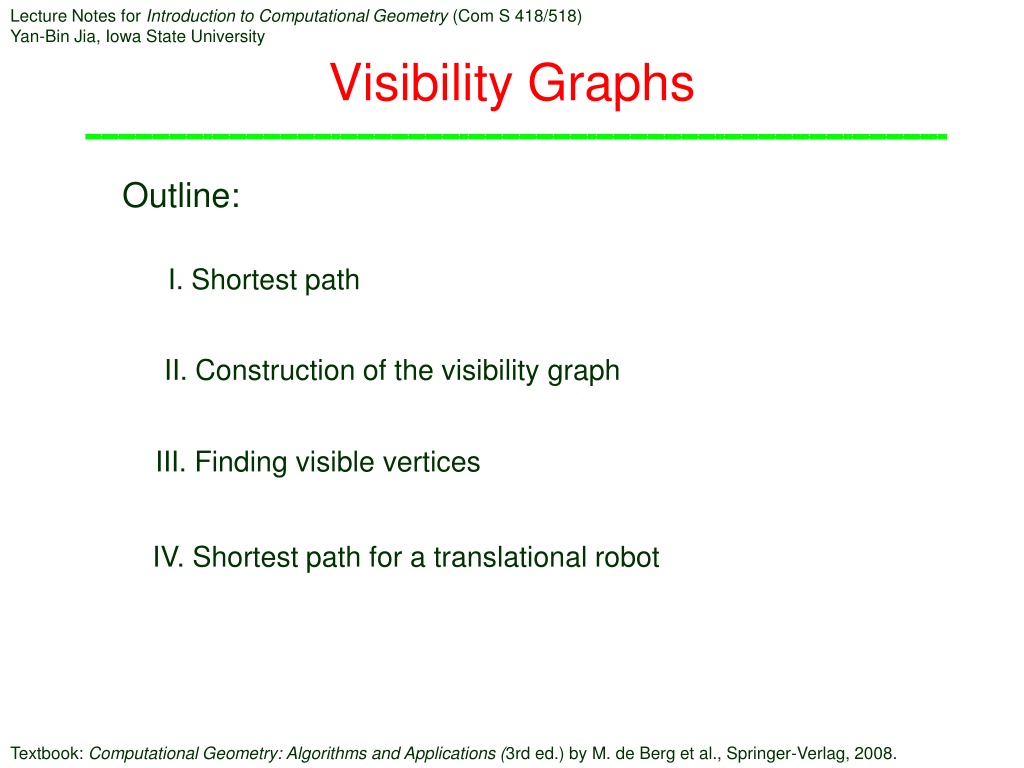
I. Shortest path
II. Construction of the visibility graph
Outline:
III. Finding visible vertices
IV. Shortest path for a translational robot
Lecture Notes for
Introduction to Computational Geometry
(Com S 418/518)
Yan-Bin Jia, Iowa State University
Textbook:
Computational Geometry: Algorithms and Applications (
3rd ed.) by M. de Berg et al., Springer-Verlag, 2008.


# degrees of freedom
of the robot

set of configurations at
which the robot collides
with the obstacle


Roadmap Construction
Motion Planning for a Point Robot
Breadth-first search over
the roadmap.
The path has smallest number of arcs from the roadmap but is often
not the shortest.
Weight each arc by its length and apply Dijkstra’s algorithm.
Still often not the shortest path length.
shortest path
Shortest Path
It has been stretched to avoid all
the obstacles.
When the band is released, it will
contract as much as possible:
following some obstacle boundaries
moving along straight segments in
the free space.
Geometry of a Shortest Path
the free space, or
an obstacle edge
II. Visibility Graph
A road map for finding the shortest path.
Shortest Path Algorithm
1. Construct the visibility graph.
3. Run Dijkstra’s algorithm.
(algorithm to be described)
Constructing the Visibility Graph
Brute-force strategy:
Test, for every pair of vertices, whether the line
segment connecting them interests any obstacle.
Improvement: Concentrate on one vertex at time to identify
all visible vertices from it.
Improved Algorithm
III. Visible Vertices from a Point
Otherwise, it is invisible.
Visibility Checking
Check visibility via binary search
over edges intersected by the ray.
rightmost edge in
the left subtree
Rotational Sweep
Algorithm for Finding Visible Vertices
Back to Visibility Checking
Take a closer look at checking if a vertex is visible during the sweep.
Non-degenerate case:
Handling Degeneracies
Pseudocode for Visibility Checking
Time on Finding All Visible Vertices
Time for Visibility Graph Construction
IV. Shortest Path for a Translational
Robot
Work space
Configuration space
Visibility graph
Shortest path
Delve into the world of Computational Geometry with a focus on Visibility Graphs and Shortest Paths, exploring concepts like Configuration Space, Roadmap Construction, Motion Planning, and the Geometry of Shortest Paths. Understand the significance of Visibility Graphs as a roadmap for determining the shortest path in a given environment. Dive deep into the principles and applications of Computational Geometry through informative lecture notes.

Download Presentation

Please find below an Image/Link to download the presentation.
The content on the website is provided AS IS for your information and personal use only. It may not be sold, licensed, or shared on other websites without obtaining consent from the author.If you encounter any issues during the download, it is possible that the publisher has removed the file from their server.
You are allowed to download the files provided on this website for personal or commercial use, subject to the condition that they are used lawfully. All files are the property of their respective owners.
The content on the website is provided AS IS for your information and personal use only. It may not be sold, licensed, or shared on other websites without obtaining consent from the author.
E N D
Presentation Transcript
Lecture Notes for Introduction to Computational Geometry (Com S 418/518) Yan-Bin Jia, Iowa State University Visibility Graphs Outline: I. Shortest path II. Construction of the visibility graph III. Finding visible vertices IV. Shortest path for a translational robot Textbook: Computational Geometry: Algorithms and Applications (3rd ed.) by M. de Berg et al., Springer-Verlag, 2008.
I. Configuration Space ? # degrees of freedom of the robot robot point ? ? ????? obstacle C-obstacle ? set of configurations at which the robot collides with the obstacle ????? ?????: union of all C-obstacles ?????: set of free configurations ????? ?????= ? ????? ?????=
Roadmap Construction Use the trapezoidal map of ?????. ?(?log?) expected time
Motion Planning for a Point Robot shortest path ???? Input: starting position ?????? goal position ????? ????? ????? ????? Breadth-first search over the roadmap. ?????? ?(?) ?????? The path has smallest number of arcs from the roadmap but is often not the shortest. Weight each arc by its length and apply Dijkstra s algorithm. Still often not the shortest path length.
Shortest Path ????? ?: a set of disjoint polygonal obstacles. Think of the path as a rubber band with endpoints fixed at ?????? and ?????. It has been stretched to avoid all the obstacles. ?????? When the band is released, it will contract as much as possible: following some obstacle boundaries moving along straight segments in the free space.
Geometry of a Shortest Path Lemma 1 The shortest path is a polygonal path whose inner vertices are also vertices of some obstacles in ?. ? ProofSuppose a shortest path ?is not polygonal. ? There exist ? ?in the free space such that ? locally is not a line segment containing ?. ? But ? can be locally shortened around ?. Contradiction. A vertex ? of ? with ? ??????, ????? cannot lie in the interior of the free space, or an obstacle edge ? Otherwise, ? can be locally shortened. ? Every inner vertex ? is an obstacle vertex.
II. Visibility Graph A road map for finding the shortest path. ????? ????(? {??????,?????}) Vertex set ? {??????,?????} Edge (?,?) exists if ? and ? can see each other it s called a visibility edge. ?????? Every obstacle edge is in ???? because its endpoints see each other. Corollary 2 The shortest path ?????? ????? consists of edges in ????.
Shortest Path Algorithm 1. Construct the visibility graph. ?(?2log?) (algorithm to be described) 2. Assign each edge ?,? the weight ?? . 3. Run Dijkstra s algorithm. = ? ?log? + ?2= ?(?2) ? ? log ? + ? Theorem 3 A shortest path ?????? ????? among a set of polygonal obstacles with ? edges can be computed in ?(?2log?) time.
Constructing the Visibility Graph It suffices to describe how to construct ????(?). Brute-force strategy: Test, for every pair of vertices, whether the line segment connecting them interests any obstacle. ?(?2) pairs ?(?) time per test ?(?3) running time Improvement: Concentrate on one vertex at time to identify all visible vertices from it.
Improved Algorithm VisibilityGraph(?) 1. ? vertices of S 2. ? 3. initialize a graph ? = (?,?) 4. for all vertices ? ? 5. do ? VisibleVertices(?,?) 6. for every vertex ? ? 7. add the edge (?,?) to ? 8. return ?
III. Visible Vertices from a Point VisibleVertices(?,?) is made no more difficult if we consider ? as a generally positioned point ? in the free space instead of a vertex of some obstacle. ? ? A vertex ? is visible from ? if ?? does not intersect the interior of any obstacle. ? Consider the half-line ? starting at ? and passing through ?. ? If ? does not hit any obstacle edge before ?, then ? is visible. Otherwise, it is invisible.
Visibility Checking Check visibility via binary search over edges intersected by the ray. ? ? Maintain the edges being intersected by ? in the balanced binary search tree ?. ?4 rightmost edge in the left subtree ? ?5 ?4 ?5 ?2 ? ?6 ?1 ?5 ?3 ? ?2 ?6 ?3 ?1 ?1 ?2 ?3 ?4 Status structure ?
Rotational Sweep Treat the vertices in cyclic order around ?. ? Sweep the plane by rotating the ray ?. At each vertex stop, ?2 ? ?4 ?3 decide if the current vertex ? is visible from ? by searching in ?; ?(log?) ?1 ?2 ? ?1 update ? by inserting/deleting obstacle edges incident to ?. ?(log?) Delete ?1 and ?2 at ?1. Insert ?3 and ?4 at ?2.
Algorithm for Finding Visible Vertices VisibleVertices(?,?) 1. sort the obstacle vertices into a list ?1,?2, ,??by polar angle with respect to ?, breaking tie by distance 2. ? half-line in the positive ?-axis direction 3. initialize a balanced BST ? to store obstacle edges intersected by ? 4. ? 5. for ? 1 to n 6. do if Visible(??) // to be described 7. then ? ? {??} 8. insert into ? incident obstacle edges at ?? that are entering the sweep line status 9. delete from ? those incident edges that are leaving the status 10. return ?
Back to Visibility Checking Take a closer look at checking if a vertex is visible during the sweep. This is carried out by Visible(??). Non-degenerate case: ?? 1 does not lie on the directed edge ??? (part of ?), i.e., ?? 1 ???. ?? ? ?? 1 ? Check if ?? is occluded by the edge ? closest to ?. ? is stored at the leftmost leaf of ?. ? ?
Handling Degeneracies Degenerate case: ?? 1 ??? ?? 1is not visible ?? 1is visible Look at ?? 1??. ?? is not visible if lies inside an obstacle (which thus must have ?? and ?? 1as vertices), or intersects an obstacle edge ? in its interior. ?? is visible otherwise. ?? is not either. ?? ? ?? 1 ? ?? 1 ?? ?? ? ? ?? ?? 1 ?? 1 ?
Pseudocode for Visibility Checking ?? Visible(??) ? 1. if ??? intersects the interior of the obstacle with ?? as a vertex 2. then return false 3. else if ? = 1 or ?? 1 is not on the segment ??? 4. then search in ? for the edge ? in the leftmost leaf 5. if ? exists and ??? intersects ? 6. then return false 7. else return true 8. else if ?? 1 is not visible 9. then return false 10. else search ? for an edge ? that intersects ???? 1 11. if ? exists 12. then return false 13. else return true ?? ? ?? 1 ? ?? ? ?? 1 ? ?(log?)
Time on Finding All Visible Vertices ?(?log?) VisibleVertices(?,?) 1. sort the obstacle vertices into a list ?1,?2, ,??by polar angle with respect to ?, breaking tie by distance 2. ? half-line in the positive ?-axis direction 3. initialize a balanced BST ? to store obstacle edges intersected by ? 4. ? 5. for ? 1 to n 6. do if Visible(??) 7. then ? ? {??} 8. insert into ? incident obstacle edges to ?? that are entering the sweep line status 9. delete from ? those incident edges that are leaving the status 10. return ? ?(?log?) ?(?log?) ?(log?) ?(log?)
Time for Visibility Graph Construction To construct the visibility graph, we call VisibleVertices() on every obstacle vertex, ??????, and ?????. ? + 2 calls ? ?log? each call Construction of the visibility graph takes? ?2log?time.
IV. Shortest Path for a Translational Robot ?: convex translational robot with constant complexity ?: a set of polygonal obstacles with ? edges in total. ? ?log2? Work space Configuration space ? ?2log? ? ?2 Shortest path Visibility graph Theorem 4 A shortest collision-free path for ? between two placements can be found in ? ?2log? time.