Understanding the Greenhouse Effect and Climate Change
Exploring the impact of greenhouse gases on Earth's climate, historical contributions of scientists, methods of measuring global temperature trends, and discussing the difference between climate and weather.
Download Presentation

Please find below an Image/Link to download the presentation.
The content on the website is provided AS IS for your information and personal use only. It may not be sold, licensed, or shared on other websites without obtaining consent from the author. Download presentation by click this link. If you encounter any issues during the download, it is possible that the publisher has removed the file from their server.
E N D
Presentation Transcript
The heat is on! Peter Guttorp peter.guttorp@nr.no guttorp@uw.edu http://www.stat.washington.edu/peter
The greenhouse effect Heat comes in from the sun Shortwave radiation Earth gets warmed up by the heat Earth radiates heat back Longwave radiation Greenhouse gases absorb much energy in radiating heat Atmosphere warms (15 C instead of -18 C) Main greenhouse gases: Water vapor Carbon dioxide Methane
The greenhouse effect Joseph Fourier (1768-1830) realized that Earth ought to be a lot cooler than it is. John Tyndall (1820-1893) found that water vapor and CO2are greenhouse gases Svante Arrhenius (1859-1927) calculated how changes in CO2can heat the planet
What is climate? Climate is what you expect; weather is what you get. Heinlein: Notebooks of Lazarus Long (1978)
Outline Measurements Models Local impact Projections
Measuring global surface temperature
Homogenization summertime correction screen painted white? miscalibrated thermometer urbanization
Global temperature measurements Marine data
Comparison between estimates Base period 1970-1989 Base period 1970-1989 Base period 1970-1989 Base period 1970-1989 Base period 1970-1989 Base period 1970-1989 0.5 0.5 0.5 0.5 0.5 0.5 0.0 0.0 0.0 0.0 0.0 0.0 Anomaly Anomaly Anomaly Anomaly Anomaly Anomaly -0.5 -0.5 -0.5 -0.5 -0.5 -0.5 -1.0 -1.0 -1.0 -1.0 -1.0 -1.0 1850 1850 1850 1850 1850 1850 1900 1900 1900 1900 1900 1900 1950 1950 1950 1950 1950 1950 2000 2000 2000 2000 2000 2000 Year Year Year Year Year Year
Is there a trend? An Ac t of Dog Global temperature
The issue of gridding Hurricanes Clouds Glaciers
Comparing global climate models to data 16 15 Simulation 14 13 12 1850 1900 1950 2000 Year Reference period 1951-1980 1.0 0.5 Anomaly ( C) 0.0 -0.5 -1.0 1880 1900 1920 1940 1960 1980 2000 Year
30-year distributions 1930-1959 1930-1959 8 300 1930-1959 CCSM4 6 HadCM3 Frequency Frequency 0.1 0.1 0.1 4 GISS data 0.0 0.0 0.0 100 2 Data Data -0.2 -0.1 -0.2 -0.1 0.6 -0.2 -0.1 0 0 -0.6 -0.2 0.2 -0.2 -0.1 0.0 0.1 -0.6 -0.4 -0.2 0.0 CMIP5 models 0.2 0.4 -0.3 -0.2 -0.1 0.0 -0.1 0.0 0.1 0.2 0.3 0.4 GISS data CMIP5 models Model Model 1970-1999 CCSM4 HadCM3 1970-1999 1970-1999 0.6 0.2 0.2 0.4 GISS data Frequency Data Data 0.2 6 0.0 0.0 Frequency 150 0.0 4 -0.2 -0.2 -0.2 0.2 0.6 1.0 0.0 0.2 0.4 0.6 -0.1 0.1 0.3 0.5 2 50 CMIP5 models Model Model 0 0 -0.4 0.0 0.4 0.8 -0.2 0.0 0.2 0.4 0.6 CMIP5 models GISS data
Comparing climate model output to weather data Global models are very coarse Regional models are driven by boundary conditions given by global model runs In either case, describes distribution of weather, not actual weather Consider a regional model driven by actual weather Stockholm 50 km x 50 km grid, 3 hr resolution (SMHI-RCA3; ERA40)
Stockholm data issues Location was moved twice (1875, 1960) Calibration (1826: 0 reads as +0.75; 1858,1915; annual thereafter)
How well does the climate model reproduce data? Observed minimum temperature 1960-2004 Regional minimum temperature 1961-2005 10 8 8 6 6 Frequency Frequency 4 4 2 2 0 0 -20 -15 -10 -5 0 -25 -20 -15 -10 -5 Temperature Temperature -5 Regional minimum daily mean -10 -15 -20 -25 -20 -15 -10 Observed minimum daily mean
Model problem? Annual average temperature over the grid square containing the Stockholm site is about 1.7 warmer than the observed average Model calculates separately open air, forest, and water/ice. Do we need finer resolution? C
Open air predictions Using 12.5 km version of RCA3, forced by ERA40, looking at only open air predictions (77% of grid square is open air) -10 -15 Model -20 -25 -25 -20 -15 -10 Observed
Is the station really in open air?
Comparison to forested model output -5 -10 Model predictions -15 -20 -25 -25 -20 -15 -10 Observed values
Why not predictions? Climate models need input of greenhouse gases, solar radiation, land use etc. To use climate models for prediction, must predict also these input variables. Instead, set up scenarios (reasonable values of the input variables). Run models with these inputs. We call that projections.
Projecting sea level rise Sea levels rise due to warming of oceans melting of land ice Most climate models do not output sea level Strategy: relate global mean temperature to global mean sea level relate global to local sea level Use projections of temperature to project local sea level
Cultural Heritage Site Storm surges up to 1.4m Land rise 2.6 mm/year Bergen Bergen 10 10 10 5 5 5 Local sea level anomaly (cm) Sea level anomaly (cm) Sea level anomaly (cm) 0 0 0 -5 -5 -5 -10 -10 -10 -15 -15 -15 -20 -20 -20 1920 1920 1940 1940 1960 1960 1980 1980 2000 2000 -10 -5 0 5 Year Year Global sea level anomaly (cm)
Components of uncertainty Bergen 2050 RCP 8.5 Bergen 2050 RCP 8.5 Bergen 2050 RCP 8.5 Bergen 2050 RCP 8.5 0.20 0.20 0.20 0.20 0.15 0.15 0.15 0.15 Density Density Density Density 0.10 0.10 0.10 0.10 0.05 0.05 0.05 0.05 0.00 0.00 0.00 0.00 0 0 0 0 10 10 10 10 20 20 20 20 30 30 30 30 40 40 40 40 Anomaly (cm) Anomaly (cm) Anomaly (cm) Anomaly (cm)
Using uncertainty in decision making Do Bergen authorities need to address sea level rise? If so, when? Adaptation costs: Outer barrier 30B NOK (5B CAD) Inner barriers 1.1B (0.2B) Need cumulative storm surge damage costs.
Current storm surge damage costs
Change due to sea level rise
Simulate damages Draw random annual cost Draw random increase factor path Draw random sea level path Accumulate costs over time Look at upper 95th percentile of cumulative costs
When is an adaptation measure beneficial? Outer barrier Inner barrier Outer barrier Inner barriers
Some references P. Guttorp and J. Xiu (2011): Climate change, trends in extremes, and model assessment for a long temperature time series from Sweden. Environmetrics 22: 456-463. P. F. Craigmile and P. Guttorp (2013): Can a regional climate model reproduce observed extreme temperatures? Statistica 73: 103-122. P. Guttorp (2014): Statistics and Climate. Annual Reviews of Statistics and its Applications 1: 87-101. P. Guttorp, D. Bolin, A. Januzzi, D. Jones, M. Novak, H. Podschwit, L. Richardson, A. S rkk , C. Sowder and A Zimmerman (2014): Assessing the uncertainty in projecting local mean sea level from global temperature. Journal of Applied Meteorology and Climatology 53: 2163-2170.
Uncertainty in cumulative damage


