Understanding Hash Tables and Hash Functions
Learn about hash tables, hash functions, collision resolution techniques like separate chaining, and how to choose the right hash function for optimal performance. Discover key concepts and methods in hashing including direct access tables, dynamic hashing/rehashing, load factors, and more.

Download Presentation

Please find below an Image/Link to download the presentation.
The content on the website is provided AS IS for your information and personal use only. It may not be sold, licensed, or shared on other websites without obtaining consent from the author. If you encounter any issues during the download, it is possible that the publisher has removed the file from their server.
You are allowed to download the files provided on this website for personal or commercial use, subject to the condition that they are used lawfully. All files are the property of their respective owners.
The content on the website is provided AS IS for your information and personal use only. It may not be sold, licensed, or shared on other websites without obtaining consent from the author.
E N D
Presentation Transcript
Hashing Alexandra Stefan 1
Hash tables Tables Direct access table (or key-index table): key => index Hash table: key => hash value => index Main components Hash function Collision resolution Different keys mapped to the same index Dynamic hashing/rehashing reallocate the table as needed If an Insert operation brings the load factor past a threshold, e.g. 0.75, double the table. Other load factors may be used If a Delete operation brings the load factor to 1/8 , half the table. Properties: Good time-space trade-off Good for: Search, insert, delete O(1) average time Not good for: Select, sort not supported, must use a different method Reading: chapter 11, CLRS (chapter 14, Sedgewick has more complexity analysis) Hash Tables and Hash Functions - youtube video 2
Example M table size. h hash function that maps a key to an index Let M = 10, h(k) = k%10 Note: 10 is a bad table size, but is used here for ease of calculation index k 0 20 1 Insert keys: 46 -> 6 15 -> 5 20 -> 0 37 -> 7 23 -> 3 25 -> 5 collision 35 -> 9 -> 2 3 23 4 Collision resolution: - Separate chaining - Open addressing - Linear probing - Quadratic probing - Double hashing 5 15 6 46 7 37 8 9 3
Hash functions M table size. h hash function that maps a key to an index We want random-like behavior: any key can be mapped to any index with equal probability. Typical functions for numeric keys: h(k,M) = k % M Best M is a prime number. (Avoid M that has a power of 2 factor, will generate more collisions). Choose M a prime number that is closest to the desired table size. If M = 2p, it uses only the lower order p bits => bad, ideally use all bits. h(k,M) = floor( ((k-A)/(B-A))* M ) Here A k<B. Simple, good if keys are random, not so good otherwise. h(k,M) = floor(M*(k*A mod 1)) , 0<A<1 (in CLRS) Good A = 0.6180339887 (the golden ratio) Useful when M is not prime (can pick M to be a power of 2) Alternative: h(k,M) = (16161 * (unsigned)k ) % M (from Sedgewick) 4
Collision Resolution: Separate Chaining = N/M (N items in the table, M table size) load factor Separate chaining Each table entry points to a list of all items whose keys were mapped to that index. Requires extra space for links in lists Lists will be short. On average, size . Preferred when the table must support deletions. Operations: Chain_Insert(T,x) - O(1) insert x in list T[h(x.key)] at beginning. No search for duplicates Chain_Delete(T,x) O(1) delete x from list T[h(x.key)] (Here x is the record so we do not need to search for it) Chain_Search(T, k) (1+ ) (both successful and unsuccessful) search in list T[h(k)] for an item x with x.key == k. 5
Separate Chaining Example: insert 25 Inserting at the beginning of the list is advantageous in cases where the more recent data is more likely to be accessed again (e.g. new students will have to visit several offices at UTA and so they will be looked- up more frequently than continuing students. Let M = 10, h(k) = k%10 index k Insert keys: 46 -> 6 15 -> 5 20 -> 0 37 -> 7 23 -> 3 25 -> 5 collision 35 9 -> 20 0 1 2 3 23 4 25 15 5 6 46 37 7 8 = 6 9
Collision Resolution: Open Addressing = N/M (N items in the table, M table size) load factor Open addressing: Use empty cells in the table to store colliding elements. M > N ratio of used cells from the table (<1). Probing examining slots in the table. Number of probes = number of slots examined. h(k,f,M) where f gives the number of failed probes/attempts: f=0,1,2, until successful hash. Linear probing: h(k,f,M) = (h1(k) + f) % M, If the slot where the key is hashed is taken, use the next available slot and wrap around the table. Very bad: primary clustering - long chains; snowball effect: the longer the chain, the higher the chance to grow 3 reshash (linear): h(k,f,M) = (h1(k,M) + 3f) %M Bad: secondary clustering - If two keys hash to the same value, they follow the same set of probes. But better than linear. Quadratic probing: h(k,f,M) = (h1(k) + c1f+ c2f2) % M, Bad: secondary clustering - If two keys hash to the same value, they follow the same set of probes. But better than linear. Double hashing: h(k,f,M) = (h1(k,M) + f* h2(k,M)) % M, h2(k,M) should NEVER be 0. (E.g. use: h2(k,M) = 1 + k%(M-1) ) Use a second hash value as the jump size (as opposed to size 1 in linear probing). Want: h2(k) relatively prime with M. (relatively prime: they have no common divisor) M prime and h2(k,M) = 1 + k%(M-1) M= 2p and h2(k,M) = odd (M and h2(k) will be relatively prime since all the divisors of M are powers of 2, thus even). See figure 14.10, page 596 (Sedgewick) for clustering produced by linear probing and double hashing. 7
Open Addressing: quadratic Worksheet M = 10, h1(k) = k%10. Table already contains keys: 46, 15, 20, 37, 23 Next want to insert 25: h1(25) = 5 (collision: 25 with 15) Index Linear Quadratic Double hashing h2(k) = 1+(k%7) Double hashing h2(k) = 1+(k%9) Linear probing - h(k,f,M) = (h1(k) + f)% M (try slots: 5,6,7,8) Quadratic probing example: - h(k,f,M) = (h1(k) + 2f+f2)% M (try slots: 5, 8) - Inserting 35(not shown in table): (try slots: 5, 8, 3,0) 0 20 20 20 20 1 2 3 23 23 23 23 h1(k) + 2f+f2 f (probe) %10 4 0 5 15 15 15 15 1 6 46 46 46 46 7 37 37 37 37 2 8 3 9 4 8 Where will 9 be inserted now (after 35)?
Open Addressing: quadratic Answers M = 10, h1(k) = k%10. Table already contains keys: 46, 15, 20, 37, 23 Next want to insert 25: h1(25) = 5 (collision: 25 with 15) Index Linear Quadratic Double hashing h2(k) = 1+(k%7) Double hashing h2(k) = 1+(k%9) Linear probing - h(k,f,M) = (h1(k) + f)% M (try slots: 5,6,7,8) Quadratic probing example: - h(k,f,M) = (h1(k) + 2f+f2)% M (try slots: 5, 8) - Inserting 35(not shown in table): (try slots: 5, 8, 3,0) 0 20 20 20 20 1 25 2 3 23 23 23 23 h1(k) + 2f+f2 f (probe) %10 4 0 5+0=5 5 5 15 15 15 15 1 5+3=8 8 6 46 46 46 46 7 37 37 37 37 2 5+8=13 3 8 25 25 5+2*3+32 = 5+15=20 3 0 9 4 9 Where will 9 be inserted now (after 35)?
Open Addressing : double hashing - Worksheet M = 10, h1(k) = k%10. Table already contains keys: 46, 15, 20, 37, 23 Try to insert 25: h1(25) = 5 (collision: 25 with 15) Quadratic probing h1(k) + 2f+f2 f (probe) %10 0 5+0=5 5 1 5+3=8 8 Double hashing example - h(k,f,M) = (h1(k) + f* h2(k)) % M Choice of h2 matters: - h2a(k) = 1+(k%7): try slots: 5, 9, - h2(25) = 1+ (25%7) = 1+ 4 = 5 => h(k,f,M) = (5 + f*5)%M => slots: 5,0,5,0, Cannot insert 25. - h2b(k) = 1+(k%9): - h2(25) = 1 + (25%9) = 1 + 7 = 8 => h(k,f,M) = (5 + f*8)%M => slots: 5,3,1,9,7,5, 2 5+8=13 3 5+2*3+32 = 5+15=20 3 0 4 Index Linear Quadratic Double hashing h2(k) = 1+(k%7) Double hashing h2(k) = 1+(k%9) 0 20 20 20 20 Double hashing 1 25 f (pro be) Index (h1(k) + f*h2a(k) )%M (5+f*5)%10 f (pro be) Index (h1(k) + f*h2b(k) )%M (5+f*8)%10 2 3 23 23 23 23 0 0 4 1 1 5 15 15 15 15 2 2 6 46 46 46 46 3 3 7 37 37 37 37 8 25 25 4 9 5 10 Where will 9 be inserted now?
Open Addressing : double hashing - Answers M = 10, h1(k) = k%10. Table already contains keys: 46, 15, 20, 37, 23 Try to insert 25: h1(25) = 5 (collision: 25 with 15) Quadratic probing h1(k) + 2f+f2 f (probe) %10 0 5+0=5 5 1 5+3=8 8 Double hashing example - h(k,f,M) = (h1(k) + f* h2(k)) % M Choice of h2 matters: - h2a(k) = 1+(k%7): try slots: 5, 9, - h2(25) = 1+ (25%7) = 1+ 4 = 5 => h(k,f,M) = (5 + f*5)%M => slots: 5,0,5,0, Cannot insert 25. - h2b(k) = 1+(k%9): - h2(25) = 1 + (25%9) = 1 + 7 = 8 => h(k,f,M) = (5 + f*8)%M => slots: 5,3,1,9,7,5, 2 5+8=13 3 5+2*3+32 = 5+15=20 3 0 4 Index Linear Quadratic Double hashing h2(k) = 1+(k%7) Double hashing h2(k) = 1+(k%9) 0 20 20 20 20 Double hashing 1 25 f (pro be) Inde x (h1(k) + f*h2a(k) )%M (5+f*5)%10 f (pro be) Index (h1(k) + f*h2b(k) )%M (5+f*8)%10 2 3 23 23 23 23 0 5 (5+0)%10=5 0 5 (5+0)%10=5 4 1 0 (5+5)%10=0 1 3 (5+8)%10=3 5 15 15 15 15 2 5 (5+2*5)%10 =15%10= 5 Cycles back to 5 => Cannot insert 25 2 1 (5+2*8)%10 =21%10= 1 6 46 46 46 46 3 9 (5+3*8)%10=29%10= 9 7 37 37 37 37 8 25 25 4 7 (5+4*8)%10=37%10= 7 3 0 (5+3*5)%10=20%10= 0 9 5 5 (5+5*8)%10=45%10= 5 Cycles back to 5 11 Where will 9 be inserted now?
Open Addressing: Quadratic vs double hashing M = 10, h1(k) = k%10. Table already contains keys: 46, 15, 20, 37, 23 Try to insert 25: h1(25) = 5 (collision: 25 with 15) Double hashing: h(k)=(h1(k)+f*h2(k) )%M where: h1(k) = k%M h2(k) = 1+(k%(M-1)) = 1+(k%9) h2(25) = 1+(25%9) = 1+7 = 8 Quadratic hashing with: 2i+i2 h(k)= (h1(k) + 2f+f2)%M where h1(k) = k%M Index Linear Quadratic Double hashing h2(k) = 1+(k%7) Double hashing h2(k) = 1+(k%9) f (pro be) Index h(k)=(h1(k)+f*h2(k) )%M = (5+f*8)%10 (for k=25) h(k)=(h1(k) + 2f+f2)%M =(5 + 2f+f2)%10 (k=25) f (probe) Index 0 20 20 20 20 1 25 0 0 2 1 1 3 23 23 23 23 2 2 4 3 3 5 15 15 15 15 4 4 6 46 46 46 46 5 7 37 37 37 37 8 25 25 Choice of h2 matters. See h2(k) = 1+(k%7) h2(25) = 1+4 = 5 => h(25) cycles: 5,0,5,0 => Could not insert 25. 9 12 Where will 9 be inserted now?
Open Addressing: Quadratic vs double hashing M = 10, h1(k) = k%10. Table already contains keys: 46, 15, 20, 37, 23 Try to insert 25: h1(25) = 5 (collision: 25 with 15) Double hashing: h(k)=(h1(k)+f*h2(k) )%M where: h1(k) = k%M h2(k) = 1+(k%(M-1)) = 1+(k%9) h2(25) = 1+(25%9) = 1+7 = 8 Quadratic hashing with: 2f+f2 h(k)= (h1(k) + 2f+f2)%M where h1(k) = k%M Index Linear Quadratic Double hashing h2(k) = 1+(k%7) Double hashing h2(k) = 1+(k%9) f (pro be) Index h(k)=(h1(k)+f*h2(k) )%M = (5+f*8)%10 (for k=25) h(k)=(h1(k) + 2f+f2)%M =(5 + 2f+f2)%10 (k=25) f (probe) Index 0 20 20 20 20 1 25 0 5 (5+0)%10=5 0 5 5+0=5 2 1 3 (5+8)%10=3 1 8 5+3=8 3 23 23 23 23 2 1 (5+2*8)%10 =31%10= 1 2 3 5+8=13 4 3 9 (5+3*8)%10=29%10= 9 5+2*3+32 = 5+15=20 3 0 5 15 15 15 15 4 7 (5+4*8)%10=37%10= 7 4 6 46 46 46 46 5 5 (5+5*8)%10=45%10= 5 Cycles back to 5 7 37 37 37 37 8 25 25 Choice of h2 matters. See h2(k) = 1+(k%7) h2(25) = 1+4 = 5 => h(25) cycles: 5,0,5,0 => Could not insert 25. 9 13 Where will 9 be inserted now?
Search and Deletion in Open Addressing Searching: Report as not found when land on an EMPTY cell Deletion: Mark the cell as DELETED , not as an EMPTY cell Otherwise you will break the chain and not be able to find elements following in that chain. E.g., with linear probing, and hash function h(k,i,10) = (k + i) %10, insert 15,25,35,5, search for 5, then delete 25 and search for 5 or 35. 14
Open Addressing: clustering Linear probing primary clustering: the longer the chain, the higher the probability that it will increase. Given a chain of size T in a table of size M, what is the probability that this chain will increase after a new insertion? Quadratic probing Secondary clustering 15
Expected Time Complexity for Hash Operations (under perfect conditions) Operation \Methods Separate chaining Open Addressing Successful search (1+ ) (1/ )ln(1/(1- )) Unsuccessful search (1+ ) 1/(1- ) Insert (1) When: insert at beginning and no search for duplicates 1/(1- ) The time complexity does not depend only on , (but also on the deleted cells). In such cases separate chaining may be preferred to open addressing as its behavior has better guarantees. Delete (1) Assumes: doubly-linked list and node with item to be deleted is given. simple uniform hashing uniform hashing Perfect conditions: Theorem 11.1 and 11.2 Theorem 11.6 and 11.8 and corollary 11.7 in CLRS Reference = N/M is the load factor 16
Perfect Hashing Like separate chaining, but use another hash table instead of a linked list. Can be done for static keys (once the keys are stored in the table, the set of keys never changes). Corollary 11.11:Suppose that we store N keys in a hash table using perfect hashing. Then the expected storage used for the secondary hash tables is less than 2N. 17
Hashing Strings Polynomial hash code (Implementation - avoid number overflow) ??? ? = ?0?1?2 ??, ?????????? ?? ???? ??? ? (??? ?????? ?? ????? [0,? 1]): ?? ? ?????? ( ??? ?0 ?? ? ? ????? ? ??????? ??? ?? ?? ? ? ???? ? ??????? ?? ? ? ??????). ??,? = ?0 ??+ ?1 ?? 1+ + ?? 1 ? + ?? 1 %? 1 ?? ????? ?? ????? ???????? ??????? ?? ??????????? ??? ????? ??? ? ?? ??? ????: ??,? = ((( ( ?0%? ? + ?1)%?) ? + ?2)%?) ? + +?? 1)%?) ? + ?? )%? (2) (Both expressions give the same value for ha(s,M) ) Recommendations: Choose a and M to be prime numbers. Recommended values for a: 33, 37,39,41 (citation: Data Structures and Algorithms in Java by Goodrich and Tamassia) E.g. h33("dog",101) =( ASCII(d)*332 + ASCII(o)*33 + ASCII(g) ) %101 = (100*1089 + 111*33+ 103)%101 = 112666 % 101 = 51 The other method: Discussion: 1) a should have some non-zero lower order bits. (Reason: If all the lower order bits of a are 0, in expression (1), when multiplying by powers of a and then truncating due to overflow, the influence of first letters of s is removed. Since expressions (1) and (2) give the same result, it means that this happens even when explicitly avoiding the overflow.) 2) If a and M have a common divisor, other issues may appear and thus a better choice is to pick a and M to be relatively prime with each other. (See a discussion here: Magic numbers in polynomial hash functions.) => Note that if both a and M are prime, then they are also prime with each other and because a is not a multiple of any power of 2 it will also have non-zero lower order bits. Magic numbers in polynomial hash functions To understand overflow, pick a = 33 > 32 = 25 the term 33t > 32t = (25)t = 25t > 232for t 7 => for strings of length 8 or more, the at term alone overflows a 4B integer (even more so after multiplying with s0 and adding the other terms). Worked-out code for s = dog Function call: hash("dog",101) M=101, s = dog (ASCII(d)=100, ASCII(o)=111, ASCII(g)=103 ) h=0, a=33 i = 0, s[0]->d : h = (33*0+100)%101 = 100 i = 1, s[1]->o : h = (33*100+111)%101=78 i = 2, s[2]->g : h = (33*78+103)%101 = 51 return 51 int hash(char *s, int M) { int i, h = 0, a = 33; for (i = 0; i<strlen(s); i++) { h = (a*h + s[i]) % M; // here s[i] will use the ASCII code } return h; } 18
Hashing strings Note that the hash function for strings given in the previous slide can be used as the initial hash function. Based on what type of hash table you have, you will need to do additional work If you are using separate chaining, you will create a node with this word and insert it in the linked list (or if you were doing a search, you would search in the linked list) If you are using open addressing: For linear, you can use at the next cells as needed For quadratic, you would use this function in the expression with the quadratic terms E.g. index = [h33( dog ,101) + 2i+i2]%101 For double hashing you will need to choose another hash function (e.g. 1+h41("dog",100) ) to get the jump size E.g. index = {h33(dog, 101) + i*[1+h41(dog,100)]}%101 19
Hash Tables in Popular Languages An Analysis of Hash Map Implementations in Popular Languages Reference: https://rcoh.me/posts/hash-map-analysis/ Chaining: Java, C++, C#, Scala, Go Open addressing: Ruby, Python HashMap in Java 8 Reference: https://www.geeksforgeeks.org/internal-working-of-hashmap-java/ In Java 8, a HashMap is implemented with separate chaining. Default load factor is 0.75 For efficiency, the bucket (chain) starts as a linked list but after a certain threshold it is replaced with a balanced tree. C++ Reference: http://www.open-std.org/jtc1/sc22/wg21/docs/papers/2013/n3690.pdf The elements of an unordered associative container are organized into buckets. Keys with the same hash code appear in the same bucket. The number of buckets is automatically increased as elements are added to an unordered associative container, so that the average number of elements per bucket is kept below a bound. Rehashing invalidates iterators, changes ordering between elements, and changes which buckets elements appear in, but does not invalidate pointers or references to elements. For unordered_multiset and unordered_multimap, rehashing preserves the relative ordering of equivalent elements. 20
% % is the remainder operator Note that if the number on the left is smaller than the number on the right, the result is the number on the left (and NOT 0; 0 is the result of the integer division in that case, but not the remainder) 7 % 10 is 7 4 % 9 is 4 48 % 13 is 9 21
Extra 22