Understanding Dynamic Regression Models and Koyck Model

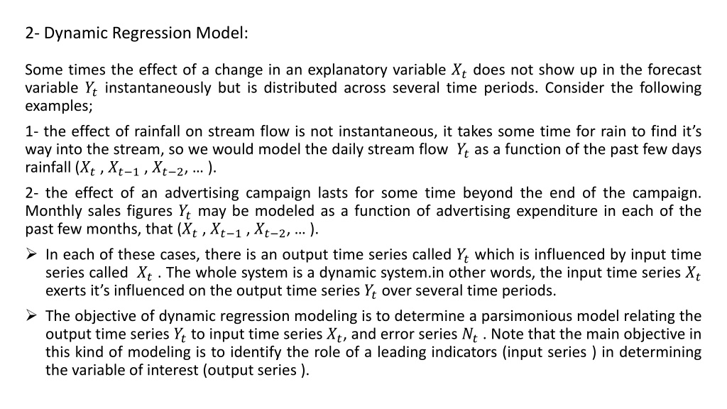
2- Dynamic Regression Model: Some times the effect of a change in an explanatory variable ??does not show up in the forecast variable ??instantaneously but is distributed across several time periods. Consider the following examples; 1- the effect of rainfall on stream flow is not instantaneous, it takes some time for rain to find it s way into the stream, so we would model the daily stream flow ??as a function of the past few days rainfall (??, ?? 1, ?? 2, ). 2- the effect of an advertising campaign lasts for some time beyond the end of the campaign. Monthly sales figures ??may be modeled as a function of advertising expenditure in each of the past few months, that (??, ?? 1, ?? 2, ). In each of these cases, there is an output time series called ??which is influenced by input time series called ??. The whole system is a dynamic system.in other words, the input time series ?? exerts it s influenced on the output time series ??over several time periods. The objective of dynamic regression modeling is to determine a parsimonious model relating the output time series ??to input time series ??, and error series ??. Note that the main objective in this kind of modeling is to identify the role of a leading indicators (input series ) in determining the variable of interest (output series ).

Lagged explanatory variables: The dynamic regression model should include not only the explanatory variable ??,but also previous values of the explanatory variables ( ?? 1, ?? 2, ) ,thus we write the dynamic regression model as following; ??= ? + ?0??+ ?1?? 1+ ?2?? 2+ + ???? ?+ ?? Where ??is an ARIMA process. The values (?0, ?1, ?2, , ??) is called the impulse response weights, or the transfer function weights, these coefficients is a measure of how the response variable ??responds to a change in ?? ?( where i= 0,1,2, ,k ) . 1 The lagged the explanatory variables are usually collinear, so that caution is needed in attributing much meaning to each coefficient,( the multicollinearity problem occurrence occurs ). Model (1) can be rewrite as following; ??= ? + (?0+ ?1? + ?2?2+ + ????)??+ ?? Or ; 2 ??= ? + ?(?)??+ ?? Where; ? ? = ?0+ ?1? + ?2?2+ + ???? 3

? ? is called the transfer function, since it describes how a change in ??is transform to ??. We call models of the form (2 or 3 ) dynamic regression models because they involve a dynamic relationship between the response and explanatory variables. In the case that (??) is white noise process ( i.e. ??~??(0,?2) ) in both eq.(1) and eq.(2 or 3 ), the model become as distributed lag model. Dynamic regression model allow current and past values of the explanatory variable ( X ) to influence the forecast variable ( Y ). How ever ( Y ) is not allowed to ( X ). There are two formulas for the dynamic regression model; 1- the basic formula which is shown in eq.(1), which is the primary model. 2- the modified formula which is shown in eq.(2 or 3) , which is the short hand relation for the dynamic model.

Koyck Model: An important dynamic regression model is the koyck model which developed by Koyck (1954). We suppose that the effect of the response variable X decrease exponentially over time, there for, let: ??= ? + ?(??+ ??? 1+ ?2?? 2+ + ???? ?) + ?? Where; ? < 1 The coefficient of ?? ?is (??= ???) which will be close to zero for large k because is smaller than one in absolute value. That is mean (? > ?2> ?3> > ??). Koyck model give large weights for close periods and smaller weights for longer periods of time. This model is some times used in modeling the response of sales to advertising expenditure since advertising in month (t) will have decreasing effect over future moths. 4 The transfer function of Koyck model has special form; ? ? = ?(1 + ?? + ?2?2+ + ????) 5 We can write the transfer function ? ? in parsimonious form as following; Multiplying both sides of eq.(5) by ( 1- B ) we get: (1 ??)? ? = ?(1 ??)(1 + ?? + ?2?2+ + ????) = ?(1 + ?? + ?2?2+ + ???? ?? ?2?2 ???? ??+1??+1)

(1 ??)? ? = ?(1 ??+1??+1) 6 And if k is large we get: (1 ??)? ? = ? So we can write the transfer function ? ? in parsimonious form as; ? (1 ??) 7 Thus we have replaced the transfer function by a more parsimonious form to get the parsimonious form for Koyck model which is; ? (1 ??)??+ ?? 8 ? ? = ??= ? +

The basic forms of the dynamic regression model: The dynamic regression model is written in two general forms. The first form is as following: ??= ? + ? ? ??+ ?? Where; ??: the forecast variable or output series. ??: the explanatory variable or input series. ??: the combined effects of all other factors influencing ??, which called Noises. ? ? = ?0+ ?1? + ?2?2+ + ???? where B is the back shift operator , i.e. ( ???= ?? 1 transfer function. The input series ??, and the output series ??should be stationary in mean and variance, and they should be appropriately transformed to take care of non-stationary variance, differenced to take care of non-stationary means, and possibly seasonally adjusted. The order of transfer function is (k) ( being the largest lag of the explanatory variable X that used ) and this can sometimes be rather large and therefore not parsimonious. So for this reason the dynamic regression model is also written in more parsimonious form, in the same way as we wrote the Koyck model in a simpler form . 9 10 ????= ?? ? ), k is the order of the or

The second form ( The parsimonious form ): The parsimonious form of the dynamic regression model is as following: ??= ? +?(?) 11 where; ?(?) = ?0+ ?1? + ?2?2+ + ???? ? ? = 1 ?1? ?2?2 ???? ??and ??as defined later. r , s , b , are constant. ??=?(?) , that is ??is an ARIMA process. The two expression, w(B) and (B) replace the v(B) expression in eq.(9), and so we get a more parsimonious model. This reduces the numbers of parameters to estimate. The order of w(B) which is (s), and that for (B) which is (r) are usually going to be much smaller than the value of (k) which is the order of the transfer function v(B)in model (9), and this reduce the number of the parameters to be estimated, making more efficient use of the data, in other word reducing the lose of the number of the observation which lead to reduce the lose in the degree of freedom. For example, in the Koyck model (the parsimonious form eq.8 ) we have s = 0 and r = 1 , so that there are fewer parameters than for model (9)where we would have needed a large value of (k) to capture the decaying effect of advertising. ?(?)?? ?+ ?? (?)??

For example, suppose w(B)= 1.2 0.5B , and (B)= 1-0.8B , then ?(?) ?(?)=1.2 0.5? 1 0.8?= 1.2 0.5? 1 0.8? 1= 1.2 0.5? (1 + 0.8? + 0.82?2+ ) = 1.2 + 0.46? + 0.368?2+ 0.294?3+ 0.236?4+ = ?(?) Which is the transfer function of the model (9), that is we would have an infinite number of terms ( infinite number of v weights), this is for ( s = 1 ) and ( r = 1 ), so we have ( k ) is very large. In eq.(11) , the subscript for X is ( t-b ), and this mean that there is a delay of (b) periods before X influence Y , so that ??influences ??+?, or ?? ?influences ??. When ( b > 0 ), X is often called a leading indicator, since ??is leading ??by b time periods. The occurrence of multicollinearity occurs due to the lagged explanatory variables in the dynamic model.

Selecting the dynamic regression model order: We will keep things simple by assuming there is just one explanatory variable, so our full model is the dynamic regression model in eq.(11), we write it again; ??= ? +?(?) ?(?)?? ?+ ?? where; ?(?) = ?0+ ?1? + ?2?2+ + ???? ??=?(?) and ? ? = 1 ?1? ?2?2 ???? (?)?? , that is ??is an ARIMA(p,d,q) process. In selecting the dynamic regression model order we need to determine the value of s and r ( the order of ?(?) and ? ? ) and the value of b (delay periods ),and the values of p , d , q in the ARMA(p,d,q) model for ??. If the data are seasonal, we may be need also to find the order of the seasonal part of ARIMA model. There are two methods which are used to select the order of dynamic regression model; The first method which is the older and more complicated method is due to Box and Jenkins ( 1970) in this method we use the prewhitening and cross-correlation. This method is difficult to use, particularly with more than one explanatory variable.

The second method; which is known as the Linear transfer function ( LTF method ). The general procedure of identifying the appropriate dynamic regression model is as follows: Step one: fit a multiple regression model of the following form, using OLS ; ??= ? + ?0??+ ?1?? 1+ ?2?? 2+ + ???? ?+ ?? Where (k) is sufficiently large so the model captures the longest time-lagged response that is likely to be important. Since the form of the noise (??) is relatively unimportant at this stage, it is convenient to use a low-order proxy AR model for (??). Step two: after estimating ??, compute ( ??= ?? ??), if the errors ( ??) from the estimated regression model appear nonstationary, and differencing appears appropriate, then difference Y and X , fit the model again using a low-order AR model for (??), in this time using differenced variables. Step three: if the errors now appear stationary, identify an appropriate transfer function for v(B), that is the values of ( b , s , r ) must be selected. The value of (b) is the number of period before (??) influences (??). The value of (s) which is the order of w(B), controls the number of transfer function coefficients before they begin to decay. The value of (r) which is the order of (B), control the decay pattern.

The following rules may be used to select the values for ( b , r , s ); 1. The dead time (b), is equal to the number of v-weights that are not significantly different from zero. That is we look for a set of approximately zero-valued v-weights (?0,?1 ?? 1) . 2. The value of (r) determines the decay pattern in the remaining v-weights; If there is no decay pattern at all but a group of spikes followed by a cut off to zero, then choose ( r=0 ). If there is a simple exponential decay ( perhaps after some v-weights that do not decay ), then choose ( r= 1). If the v-weights show a more complex decay pattern ( i.e. damped sine-wave decay ) then ( r=2 ) . 3. The value of (s) is the number of non-zero v-weights before the decay. Step four: calculate the errors from the estimated regression model; ??= ?? ? + ?0??+ ?1?? 1+ ?2?? 2+ + ???? ? And identify an appropriate ARMA model for the error series. Step five: refit the entire model using the new ARMA model for the error and the transfer function for X .

Step sex: finally, we need to check that the fitted model is adequate by analysis the residual ( ??) to see if they are significantly different from a white noise series. The usual diagnostic test which is in ARIMA model can be used. Note that, a wrong dynamic regression model may induce significant autocorrelations in the residuals. If the residuals show any problems, it is good practice to reconsider the appropriateness of the transfer function as will as the error model. Forecasting: Once the model has been identified and all the parameters have been estimated, the forecasting version of the equation needs to determined. We first rewrite the dynamic regression model (11) in single equation by replacing ??by it s operator form; ??= ? +?(?) 12 Where ??is white noise , we assumed that ??has stationary ARMA model, if not all variables must be differenced first. Eq. 12 multiply by the product of ?(?) and (?), we get: ?(?) (?)??= ?(?) (?)? + (?)?(?)?? ?+ ?(?)?(?)?? Using the estimated values of the parameters, past values of ( Y , X , e ) , and the future values of (X and e ), we can determine the future values of Y . If X is not random but under the control, so we can used the fixed values of X ( past and future ) in making forecasts about Y. when X is random, it is common to forecast X as an ARIMA process and to feed the forecasts of X obtained in this way into the forecasting equation. ?(?)?? ?+?(?) (?)?? 13