Understanding Differential Equations in Physical Phenomena
Differential equations play a crucial role in modeling physical phenomena involving rates of change like fluid motion, mechanical systems, and heat dissipation. This content explores examples of differential equations in motion and provides insights on sketching direction fields using tools like Maple and Matlab.
Download Presentation

Please find below an Image/Link to download the presentation.
The content on the website is provided AS IS for your information and personal use only. It may not be sold, licensed, or shared on other websites without obtaining consent from the author. Download presentation by click this link. If you encounter any issues during the download, it is possible that the publisher has removed the file from their server.
E N D
Presentation Transcript
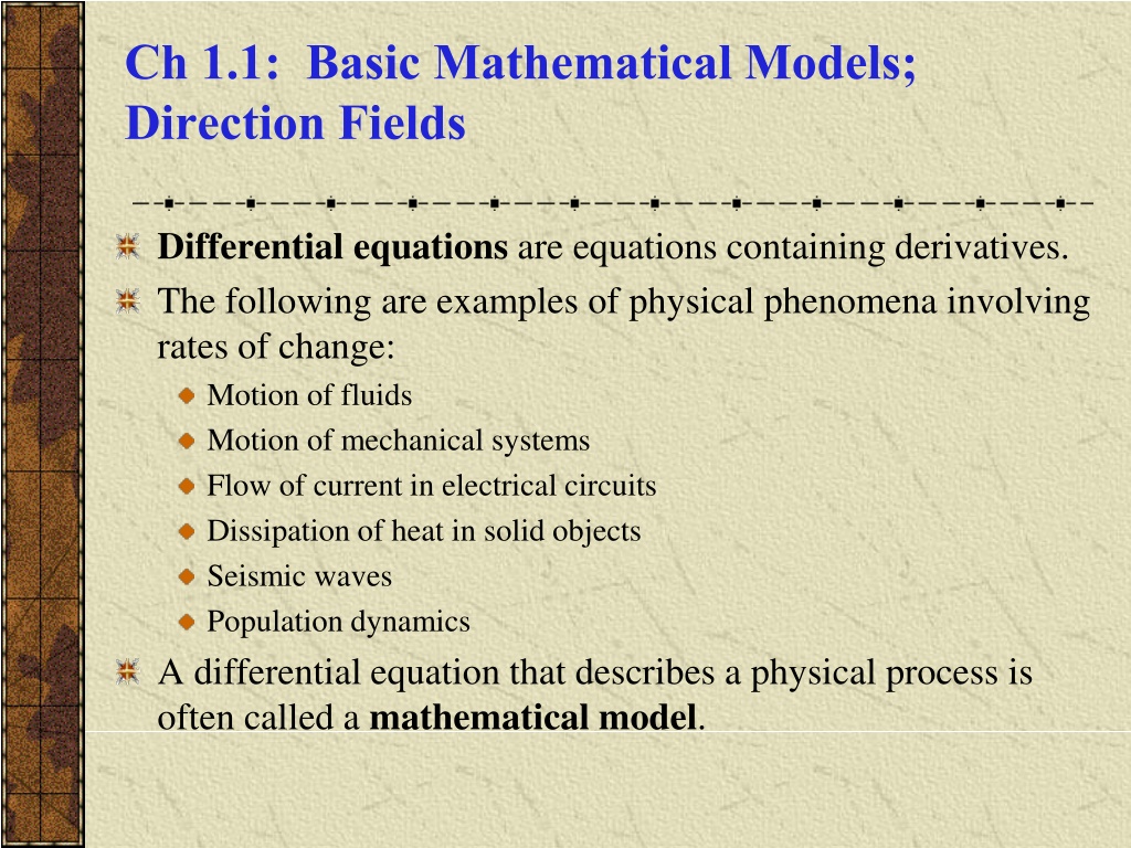
Ch 1.1: Basic Mathematical Models; Direction Fields Differential equations are equations containing derivatives. The following are examples of physical phenomena involving rates of change: Motion of fluids Motion of mechanical systems Flow of current in electrical circuits Dissipation of heat in solid objects Seismic waves Population dynamics A differential equation that describes a physical process is often called a mathematical model.
Example 1: Free Fall Formulate a differential equation describing motion of an object falling in the atmosphere near sea level. Variables: time t, velocity v Newton s 2ndLaw: F = ma = m(dv/dt) net force Force of gravity: F = mg Force of air resistance: F = v upward force Then v mg dt downward force dv = m Taking g = 9.8 m/sec2, m = 10 kg, = 2 kg/sec, we obtain dv 2 . 0 8 . 9 = v dt
= 8 . 9 2 . 0 v v Example 2: Sketching Direction Field (1 of 3) Using differential equation and table, plot slopes (estimates) on axes below. The resulting graph is called a direction field. (Note that values of v do not depend on t.) v 0 5 10 15 20 25 30 35 40 45 50 55 60 v' 9.8 8.8 7.8 6.8 5.8 4.8 3.8 2.8 1.8 0.8 -0.2 -1.2 -2.2
8 . 9 = 2 . 0 v v Example 2: Direction Field Using Maple (2 of 3) Sample Maple commands for graphing a direction field: with(DEtools): DEplot(diff(v(t),t)=9.8-v(t)/5,v(t), t=0..10,v=0..80,stepsize=.1,color=blue); When graphing direction fields, be sure to use an appropriate window, in order to display all equilibrium solutions and relevant solution behavior.
8 . 9 = 2 . 0 v v Example 2 BIS Direction Field Using Matlab (2 of 3) Sample Matlab commands for graphing a direction field: >> [t,y]=meshgrid(0:.4:10, 0:3:80); dy=9.8-(y./5); dt=ones(size(dy));dtu=dt./sqrt(dt.^2+dy.^2); dyu=dy./sqrt(dt.^2+dy.^2); quiver(t,y,dtu,dyu, .5, 'r') When graphing direction fields, be sure to use an appropriate window, in order to display all equilibrium solutions and relevant solution behavior.
8 . 9 = 2 . 0 v v Example 2: Direction Field & Equilibrium Solution (3 of 3) Arrows give tangent lines to solution curves, and indicate where soln is increasing & decreasing (and by how much). Horizontal solution curves are called equilibrium solutions. Use the graph below to solve for equilibrium solution, and then determine analytically by setting v' = 0. = Set 0 : v 2 . 0 = 8 . 9 0 v 8 . 9 = v 2 . 0 = 49 v
Equilibrium Solutions In general, for a differential equation of the form ay y = , b find equilibrium solutions by setting y' = 0 and solving for y: b t y = ) ( a Example: Find the equilibrium solutions of the following. 5 2 = = y y y y + = + 3 ( ) 2 y y y
Example 3: Mice and Owls (1 of 2) Consider a mouse population that reproduces at a rate proportional to the current population, with a rate constant equal to 0.5 mice/month (assuming no owls present). When owls are present, they eat the mice. Suppose that the owls eat 15 per day (average). Write a differential equation describing mouse population in the presence of owls. (Assume that there are 30 days in a month.) Solution: 450 5 . 0 = p dt dp
Example 3 (Cont.): Direction Field (2 of 2) Discuss solution curve behavior, and find equilibrium soln. = 5 . 0 450 p p
Example 3 BIS: Matlab >> [t,y]=meshgrid(0:2:10, 800:20:1000); dy=0.5*y-450; dt=ones(size(dy));dtu=dt./sqrt(dt.^2+dy.^2); dyu=dy./sqrt(dt.^2+dy.^2); quiver(t,y,dtu,dyu, 'r')
Steps in Constructing Mathematical Models Using Differential Equations Identify independent and dependent variables and assign letters to represent them. Choose the units of measure for each variable. Articulate the basic principle that underlies or governs the problem you are investigating. This requires your being familiar with the field in which the problem originates. Express the principle or law in the previous step in terms of the variables identified at the start. This may involve the use of intermediate variables related to the primary variables. Make sure each term of your equation has the same physical units. The result may involve one or more differential equations.
