Understanding Algorithm Analysis and Scalability in Computer Science

Scientists and computer scientists often encounter scale differences, and scalability is crucial for accommodating growing inputs. Algorithm analysis, data structures, running times, and experimental studies are key aspects explored in the context of algorithms. Choosing the right type of plot for linear, polynomial, and exponential growth is also discussed.

• Algorithm Analysis
• Scalability
• Data Structures
• Running Times
• Experimental Studies

tuuli Follow

Uploaded on Apr 20, 2024 | 4 Views

Download Presentation

Please find below an Image/Link to download the presentation.

The content on the website is provided AS IS for your information and personal use only. It may not be sold, licensed, or shared on other websites without obtaining consent from the author. Download presentation by click this link. If you encounter any issues during the download, it is possible that the publisher has removed the file from their server.

Presentation Transcript

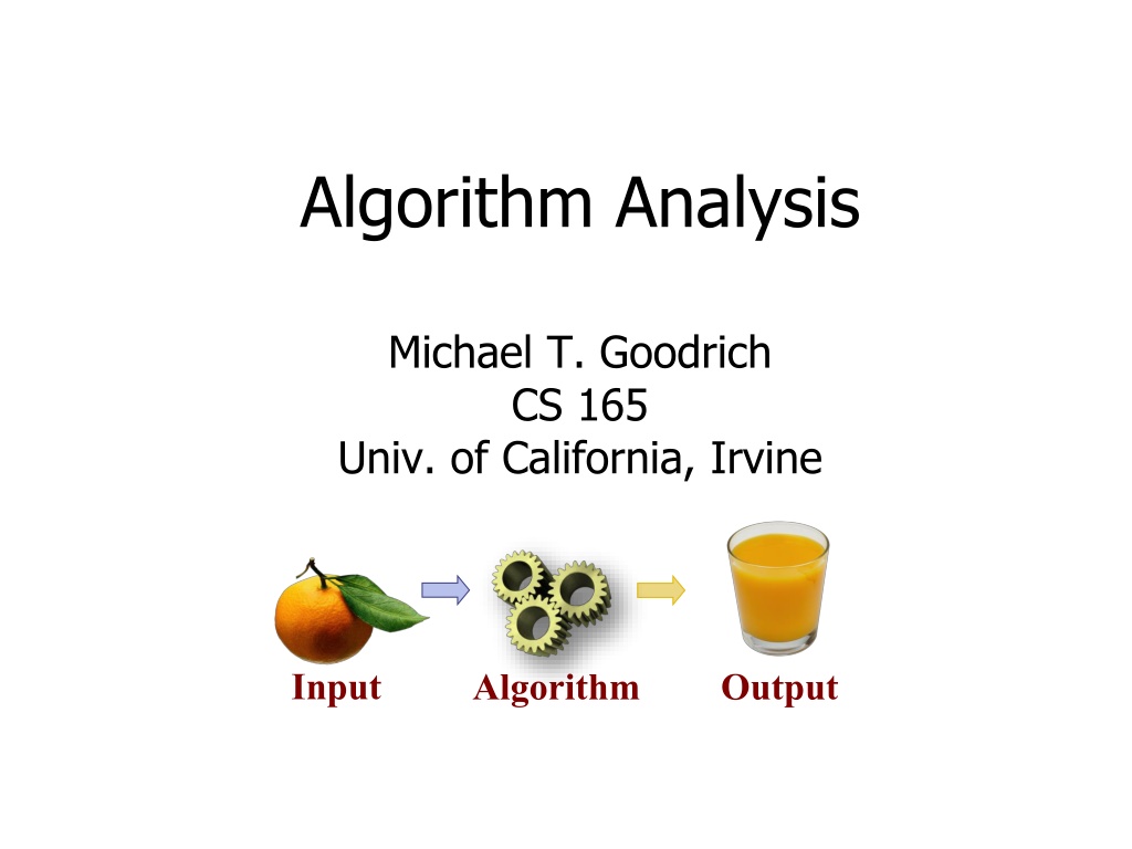
1. Algorithm Analysis Michael T. Goodrich CS 165 Univ. of California, Irvine Input Algorithm Output

2. Scalability Scientists often have to deal with differences in scale, from the microscopically small to the astronomically large. Computer scientists must also deal with scale, but they deal with it primarily in terms of data volume rather than physical object size. Scalability refers to the ability of a system to gracefully accommodate growing sizes of inputs or amounts of workload. Algorithm Analysis 2

3. Algorithms and Data Structures An algorithm is a step-by-step procedure for performing some task in a finite amount of time. Typically, an algorithm takes input data and produces an output based upon it. Input Algorithm Output A data structure is a systematic way of organizing and accessing data. Algorithm Analysis 3

4. Running Times Most algorithms transform input objects into output objects. The running time of an algorithm typically grows with the input size. Average case time is often difficult to determine. We focus primarily on the worst case running time. Theoretical analysis Might not capture real-world performance best case average case worst case 120 100 Running Time 80 60 40 20 0 1000 2000 Input Size 3000 4000 Algorithm Analysis 4

5. Experimental Studies 9000 8000 7000 Write a program implementing the algorithm Run the program with inputs of varying size and composition, noting the time needed: Plot the results Try to match a curve to the times 6000 Time (ms) 5000 4000 3000 2000 1000 0 0 50 100 Input Size Algorithm Analysis 5

6. Choose the Right Type of Plot Linear growth Algorithm Analysis 6 Image from https://medium.com/@scajanus/types-of-growth-and-how-to-show-them-4de77918dc2e

7. Choose the Right Type of Plot Polynomial growth Algorithm Analysis 7 Image from https://medium.com/@scajanus/types-of-growth-and-how-to-show-them-4de77918dc2e

8. Choose the Right Type of Plot Exponential growth Algorithm Analysis 8 Image from https://medium.com/@scajanus/types-of-growth-and-how-to-show-them-4de77918dc2e

9. Seven Important Functions Seven functions that often appear in algorithm analysis: Constant 1 Logarithmic log n Linear n N-Log-N n log n Quadratic n2 Cubic n3 Exponential 2n 1E+30 1E+28 Cubic 1E+26 Quadratic 1E+24 1E+22 Linear 1E+20 1E+18 T (n ) 1E+16 1E+14 1E+12 1E+10 1E+8 1E+6 1E+4 In a log-log chart, the slope of the line corresponds to the exponent in the growth rate 1E+2 1E+0 1E+0 1E+2 1E+4 1E+6 1E+8 1E+10 n Algorithm Analysis 9

10. Slope in a log-log plot The reason the slope of a straight line in a log-log plot corresponds to the exponent in the running time: y = nc log y = log nc log y = c*log n Algorithm Analysis 10

11. Slide by Matt Stallmann included with permission. Why Growth Rate Matters if runtime is... time for n + 1 time for 2 n time for 4 n c lg n c lg (n + 1) c (lg n + 1) c(lg n + 2) c n c (n + 1) 2c n 4c n runtime quadruples when problem size doubles ~ c n lg n + c n 2c n lg n + 2cn 4c n lg n + 4cn c n lg n c n2 ~ c n2 + 2c n 16c n2 4c n2 c n3 ~ c n3 + 3c n2 8c n3 64c n3 c 2n c 2 n+1 c 2 2n c 2 4n Algorithm Analysis 11

12. Constant Factors (log-log plot) 1E+26 Quadratic Quadratic Linear Linear The growth rate is minimally affected by constant factors or lower-order terms Examples 102n+ +105is a linear function 105n2+ + 108nis a quadratic function 1E+24 1E+22 1E+20 1E+18 1E+16 1E+14 T(n) 1E+12 1E+10 1E+8 1E+6 1E+4 1E+2 1E+0 1E+0 1E+2 1E+4 1E+6 1E+8 1E+10 n Algorithm Analysis 12

13. Big-Oh Notation 10,000 Given functions f(n) and g(n), we say that f(n) is O(g(n)) if there are positive constants c and n0 such that f(n) cg(n) for n n0 Example: 2n+10 is O(n) 2n+10 cn (c 2) n 10 n 10/(c 2) Pick c = 3 and n0 = 10 3n 2n+10 1,000 n 100 10 1 1 10 100 1,000 n Algorithm Analysis 13

14. Big-Oh Example 1,000,000 n^2 100n 10n n Example: the function n2is not O(n) n2 cn n c The above inequality cannot be satisfied since c must be a constant 100,000 10,000 1,000 100 10 1 1 10 100 1,000 n Algorithm Analysis 14

15. Big-Oh Rules If is f(n) a polynomial of degree d, then f(n) is O(nd), i.e., 1. Drop lower-order terms 2. Drop constant factors Use the smallest possible class of functions Say 2n is O(n) instead of 2n is O(n2) Use the simplest expression of the class Say 3n+5 is O(n) instead of 3n+5 is O(3n) Algorithm Analysis 15

16. Relatives of Big-Oh big-Omega f(n) is (g(n)) if there is a constant c > 0 and an integer constant n0 1 such that f(n) c g(n) for n n0 big-Theta f(n) is (g(n)) if there are constants c > 0 and c > 0 and an integer constant n0 1 such that c g(n) f(n) c g(n) for n n0 Algorithm Analysis 16

17. Intuition for Asymptotic Notation big-Oh f(n) is O(g(n)) if f(n) is asymptotically less than or equal to g(n) big-Omega f(n) is (g(n)) if f(n) is asymptotically greater than or equal to g(n) big-Theta f(n) is (g(n)) if f(n) is asymptotically equal to g(n) Algorithm Analysis 17