The Law-Gold model
Explore the intricate workings of sensory representation, individual neuron modeling, interneuron correlations, decision variable construction, and reinforcement learning in neuronal populations. Gain insights into how neuronal responses are pooled to form decision variables used for creating weighted predictions based on trial outcomes.
Download Presentation

Please find below an Image/Link to download the presentation.
The content on the website is provided AS IS for your information and personal use only. It may not be sold, licensed, or shared on other websites without obtaining consent from the author.If you encounter any issues during the download, it is possible that the publisher has removed the file from their server.
You are allowed to download the files provided on this website for personal or commercial use, subject to the condition that they are used lawfully. All files are the property of their respective owners.
The content on the website is provided AS IS for your information and personal use only. It may not be sold, licensed, or shared on other websites without obtaining consent from the author.
E N D
Presentation Transcript
The Law-Gold model CS786 4thMarch 2022
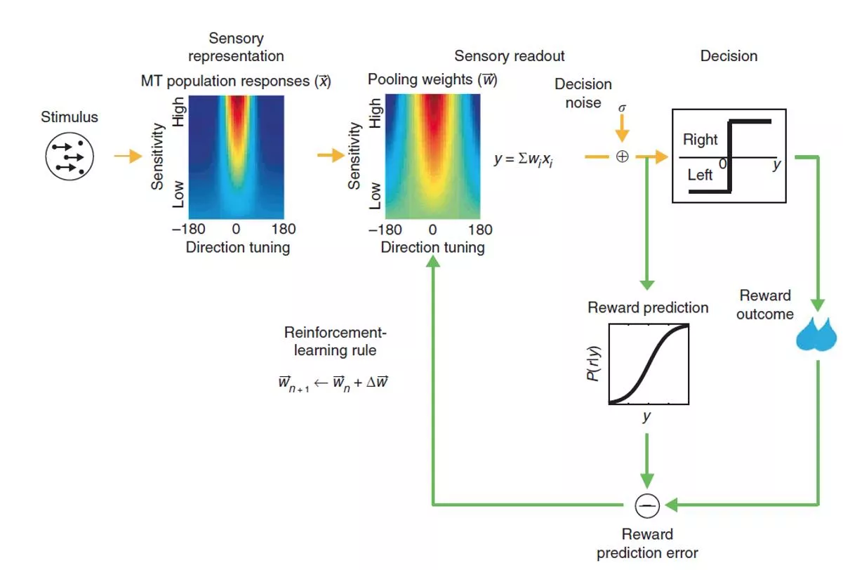
The model (Law & Gold, 2009)
Sensory representation MT modeled as a population of 7200 neurons 200 for each of 36 evenly spaced directions in the 2D plane Trial-by-trial stimulus responses fixed using neuronal data
Individual neuron model Each neuron s response to a given stimulus modeled as Gaussian with mean m k0is spiking response at 0% coherence knis spiking response at 100% coherence in null direction kpis spiking response at 100% coherence in preferred direction COH is coherence as a fraction is the neuron s preferred direction
Interneuron correlations Neurons with shared direction tuning should fire frequently together Equally excitable neurons should fire frequently together So neuron spiking rates should be correlated, based on similarity in directional tuning motion sensitivity
Decision variable construction Variable constructed by pooling neuronal responses
Pooled neuronal responses Construct a 7200 bit vector x Here, r = Uz, z ~ N(0,1) and U is the square root of the correlation matrix All neuron responses pooled to yield decision variable corrupted by decision noise
The magic sauce: weight learning Using reinforcement learning
Reinforcement learning in neurons Prediction error C is -1 for left, +1 for right r is whether there was success or not on the trial E[r] is the predicted probability of responding correctly given the pooled MT responses y x is the vector of MT responses E[x] is the vector of baseline MT responses M = 1, n = 0 for the most successful rule
How did the tuning weights vary? Graph plots neuron weights on y-axis and directional tuning on x-axis This plot shows the optimal weights to discriminate motion directions 180 degrees apart Some neurons (not all) learn that direction 0 should get high positive weights and direction 180 should get high negative weights
Perceptual learning is hyper-specific Training with horizontal Vernier scales can improve discrimination threshold 6-fold But horizontal training does not translate to vertical direction
Training specificity predictions Infrequently seen directions show less learning
Model predicts differential sensitization Sensory-motor association Perceptual sensitivity
The model (Law & Gold, 2009)
Perceptual learning as decision-making (Gold & Ding, 2013)


