Terrain Density Estimation Methods and Principles
Principles and methods for estimating terrain density, including the Parasnis method, first-difference and multiscale first-difference methods, bias in terrain density estimates, correlation with subsurface structure, wet and dry densities, and more.

Uploaded on Feb 23, 2025 | 0 Views
Download Presentation

Please find below an Image/Link to download the presentation.
The content on the website is provided AS IS for your information and personal use only. It may not be sold, licensed, or shared on other websites without obtaining consent from the author.If you encounter any issues during the download, it is possible that the publisher has removed the file from their server.
You are allowed to download the files provided on this website for personal or commercial use, subject to the condition that they are used lawfully. All files are the property of their respective owners.
The content on the website is provided AS IS for your information and personal use only. It may not be sold, licensed, or shared on other websites without obtaining consent from the author.
E N D
Presentation Transcript
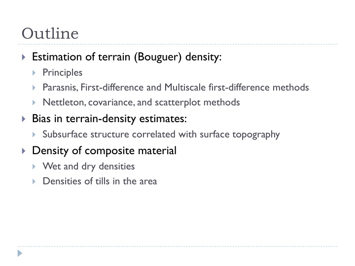
Outline Estimation of terrain (Bouguer) density: Principles Parasnis, First-difference and Multiscale first-difference methods Nettleton, covariance, and scatterplot methods Bias in terrain-density estimates: Subsurface structure correlated with surface topography Density of composite material Wet and dry densities Densities of tills in the area
Principles of terrain density estimation Optimal terrain density leads to the removal of the effect of the topography in the Bouguer-corrected gravity Bouguer-corrected gravity is due to deeper sources It is smoother It may be uncorrelated or correlated with topography Consequently, optimal density will achieve: Lower correlation of topographic elevation with Bouguer gravity Smoothest Bouguer gravity variation
Variance reduction and correlation Note that the variance ( 2) is the squared mean statistical error: The variances due to subsurface anomalies (those we are interested in) and to the surface topography (those we want to get rid of) are additive in the data : ( ) ( ) 2 2 = 2 g g g ( ( ) 2 = + = 2 g g anomaly topo ) ( ) 2 2 = + + = 2 g g g g anomaly topo anomaly topo This is the covariance. These anomalies should not be correlated (< >=0) = 2 anomaly + 2 topo So, if we manage to remove the effect of topography in Bouguer gravity gB, we likely reduce its 2
Parasnis method Cross-plot the values of scaled free-air gravity gFA/2 G versus elevationh(x) Criterion for selecting : the points (h, gFA/2 G) should fall on a straight line The slope of this line equals density There may be several such lines corresponding to different rocks (say, near-surface tills and underlying shale)
The method of first differences Calculate ratios gFA /2 G h(x) of the differences of free-air gravity gFA to elevation differences h(x) for adjacent stations Criterion for selecting : all these ratios should equal
Multi-scale first differences Calculate ratios app = gFA / h/2 G( apparent density ) for many pairs of stations in an area Draw a histogram p( app) Criterion for selecting : the histogram will have peaks (most frequently occurring ratios gFA / h) at the true values of
Nettleton method The difference between this and the following methods from Parasnis and first differences is in using Bouguer instead of free-air corrected data Graphical correlation between distance variations of the Bouguer-corrected gravity gB(x) and topography h(x) Criterion for selecting : if (in Bouguer correction) is selected correctly, variations in gB(x) will be shorter-range than h(x)
Covariance method Criterion for selecting : the mean-square demeaned Bouguer anomaly gB(x)must have the smallest values Demeaned ( detrended in Jim s notes) means that the spatial average values are subtracted from both free-air gravity gFA(x) and elevation h(x) ( or from Bouguer gravity gB(x) = gFA(x) 2 Gh(x) )
Scatter plot method For each line and for some estimate of : 1) Calculate gB from gFA and h 2) Subtract linear trends from gB and h You can use Matlab s function polyfit to do this 3) Make a cross-plot (scatterplot) of these detrended (h,gB) You will see a cloud of points Calculate the correlation coefficient (r, next slide) Criterion for selecting the : the cloud must be horizontal and the covariance equal zero If r > 0 (positive slope), the is too low (under-corrected) If r < 0 (negative slope), the is too high (over-corrected) You can again measure the slope using polyfit Note that this method only looks at the covariances of small perturbations in (h,gB) but ignores the general trends 4)
Correlation coefficient Correlation coefficient between two series {x} and {y}: n n ( )( ) ( )( ) ) x x y y x x y y i i i i = = = = r 1 1 i i ( xy 1 n s s n n ( ) ( ) 2 2 x y x x y y i i = = 1 1 i i where <x> and <y> are the sample means and sx and sy are the standard deviations