Signal Resampling & Digital Filter Implementation

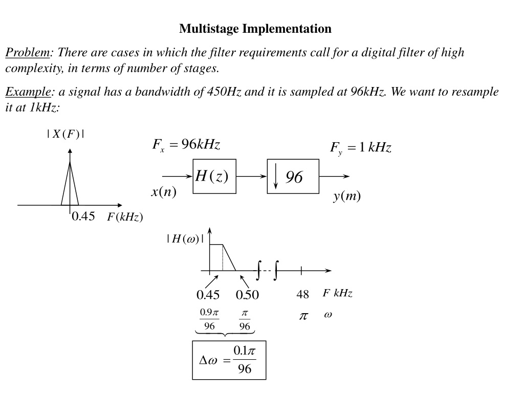
Multistage Implementation Problem: There are cases in which the filter requirements call for a digital filter of high complexity, in terms of number of stages. Example: a signal has a bandwidth of 450Hz and it is sampled at 96kHz. We want to resample it at 1kHz: | ( )| X F x= 96 F kHz y=1 F kHz ( ) H z 96 x n ( ) y m ( ) 045 . ( ) F kHz ( )| H | F kHz 045 . 09 96 050 . 96 =01 96 48 . .

Solution: for an FIR filter designed by the window method, the order of the filter is determined by the size of the transition region. With a Hamming Window the order is determined by the equation 8 M 01 96 . = = M = = 960 8 7 680 , which yields Disdvantage: a lot of computations at a high freq. rate 7 680 96 000 , = 074 109 . , /sec multiplies

One Stage Implementation: we decimate in one shot. F D x F = x F y LPF D x n ( ) y m ( ) Multistage Implementation: we decimate the signal in several stages. F D = x F x= F F y 1 F2 F3 FL x n ( ) D2 D D 1 DL D1 H2 HL H1 ( ) y m DL = D 2

See the last stage first: L( ) x n y m ( ) F D F D FL HL DL = = L x F y L H ( ) L p D L / 2 F F y F p Passband: 0 F p F F D F F y = = = 2 F L Stopband: , since / 2 y F / 2 F L 2 2 D L L L / 2 y F This filter clears everything above .

Hi Problem: we can design the low pass filters in a clever way, by taking into consideration that the spectrum is bandlimited. ( ) X [ ] 1[ ] m + ix ix n F D Fi Hi Di += 1 i F i i i X ( ) 1( ) + i X pass stop y F aliased 2 y F Fi+1 2 F y F Fi+1 Fi+1 2 Fi 2 F 2 2 iD

Hi Problem: we can design the low pass filters in a clever way, by taking into consideration that the spectrum is bandlimited. ( ) X x n i+1( ) x m i( ) F D Fi Hi Di += 1 i F i i : ( ) H 0 Fp F F Hi Specs for i pass: + 2 2 F stop: 1 i y i Fi 2 F F Fp y F+ 1 i 2

Pass Band Stop Band Sampling Freq. [0, 450] Hz > 500 Hz 96 kHz Example: same problem we saw before: Use Multistage. = = = 96 12 2 F kHz F kHz F kHz = kHz 1 F 2 3 1 4 H3 H2 H1 6 2 8 x n ( ) y m ( ) F kHz 050 . 045 . 09 2 01 . 045 . 09 12 21 12 46 15 . 3 12 . 045 . 09 96 221 96 35 115 . 23 96 . . . rad . 2 rad 2 160 order M 05 106 . 03 106 . mult./sec 34 106 .

Efficient Multirate Implementation Goal: we want to determine an efficient implementation of a multirate system. For example in Decimation and Interpolation: ) (n s (n ) x (m ) y (z ) H D (mD ) s you have to compute only, ie. one every D samples. (n ) (m ) x y (z ) H I (m ) s most of the values of s(mD) are zero

Noble Identities: (n ) (n ) x x (m ) (m ) y y (z ) G D D D ( ) G z k = ( ) ( ) ( ) y m mD g k x k = ( ) ( ) ( ) y m g m x D D = 0 if k D = ( ) ( ) ( ) y m g mD D x D D (m ) g ( ) g 2n = 2 ( 2 ) ( ) g m g m m 1 n 1 2z ( ) G (z ) G

For example take an FIR Filter x n ( ) y m ( ) x n ( ) y m ( ) h( ) 0 h( ) 0 D D z 1 D z h( ) 1 h( ) 1 z 1 D z h( ) 2 h( ) 2 since D z 1 D D z

Similarly: (n ) x (n ) (m ) (m ) y x y (z ) G M M M ( ) G z = = ( ) ( ) if g k x k m M k = ( ) ( ) ( ) y m g m kM x k ( ) y m k M otherwise 0 = 0 if m M ( ) = = ( ) ( ) if g k M x k m M M ( ) y m otherwise 0 (m ) g ( ) g 2n = 2 ( 2 ) ( ) g m g m 1 m 1 n 2z ( ) G (z ) G

x n ( ) y m ( ) x n ( ) y m ( ) h( ) 0 h( ) 0 M M z 1 M z h( ) 1 h( ) 1 z 1 M z h( ) 2 h( ) 2 since M M z 1 M z

Application: POLYPHASE Filters x n ( ) y m ( ) H z ( ) 2 Decimator: take, for example, D=2 = = + + 2 1 2 n m m ( ) h n z ( ) h m z ( 2 ) h m ( 2 1 ) H z z z n m m = + 2 1 2 ( ) ( ) ( ) H z H z e z H z o even odd

x n ( ) Therefore this system becomes: 2 e( ) H z y m ( ) z 1 2 o( ) H z 2 x n ( ) 2 e( ) H z 2 Filtering at High Sampling Rate z 1 y m ( ) 2 o( ) H z 2 Filtering at Low Sampling rate x n ( ) e( ) H z 2 z 1 y m ( ) o( ) H z 2

Similarly: x n ( ) x n ( ) y m ( ) 2 ( ) H z 2 H z ( ) 2 o z 1 y m ( ) 2 ( ) H z e x n ( ) Filtering at High Sampling Rate ( ) H z 2 o z 1 y m ( ) ( ) H z 2 e Filtering at Low Sampling Rate

Example: Consider the Filter/Decimator structure shown below, with (n ) s (n ) x (m ) y 2 . 1 = 6 . 0 + 5 . 1 + 0 . 2 + 1 2 3 4 ( ) 4 H z z z z z (z ) 2 H 0 . 2 5 . 1 + 6 . 0 + 2 . 1 + 5 6 7 8 z z z z 2 ( ) H z 2 . 1 + 5 . 1 2 + 4 z 4 5 . 1 + z + 6 2 . 1 + z 8 e 1 This can be written as = + + ( ) H z + z 2 4 6 6 . 0 0 . 2 0 . 2 6 . 0 z z z z ( H o ) 2 z and implemented in Polyphase form: x n ( ) 2 5 . 1 + + 5 . 1 + 2 . 1 + 1 2 3 4 2 . 1 4 z z z z z 1 y m ( ) 0 . 2 6 . 0 + 1 2 3 6 . 0 2 z z z 2

General Polyphase Decomposition Given any integer N: + + 1 N ( ) = = + n Nk [ ] h n z [ ] H z z h kN z = = = 0 n k ( ) N H z ( ) z ( ) z ( ) z ) 1 = + + + 1 ( N N N N ( ) ... H z H z H z H 0 1 1 N Example: take N=3 = 5 . 3 . + 2 . 4 6 . 0 + 4 . 1 2 . 0 7 . 0 + 1 2 3 4 5 6 7 ( ) 1 . 2 H z z z z z z z z = = = 2 . 4 + 3 3 6 ( ) 1 . 2 2 . 0 H z z z 0 + 3 3 6 ( ) 5 . 6 . 0 7 . 0 H z z z 1 3 3 ( ) 3 . 4 . 1 H z z 2

Apply to Downsampling ( ) z N [m y ] H [n x ] POLYPHASE ( ) N H z 1 N 1 z ( ) N H z 2 1 z ( ) N H z 1 1 z [n x ] [m y ] ( ) N N H z 0

apply Noble Identity N ( ) z H 1 N 1 z ( ) z N H 2 1 z ( ) z N H 1 1 z [n x ] [m y ] ( ) z N H 0

Serial to Parallel (Buffer) N = + 1[ ] m [( 1) 1] N x x m N 1 z N = 1[ ] x m [ 1] x mN 1 z [n x ] N = 0[ ] x m [ ] x mN Serial to Parallel (Buffer): 1[ ] m N x [n x ] 1 3 5 S/P 1 2 3 4 5 6 2 4 6 N [ ] 0m x = = 0 n n N m = 0

Same for Upsampling ( ) z N H [n x ] [m y ] POLYPHASE ( ) z [n x ] N [m y ] N H0 1 z ( ) z N H1 1 z ( ) z N H 1 N

apply Noble Identity ( ) z N [n x ] H [m y ] NOBLE IDENTITY [n x ] ( ) z [m y ] H0 N 1 z ( ) z H1 N 1 z ( ) z HN 1 N

Parallel to Serial (Unbuffer or Interlacer) N [ ] y m [ ] y 0n 1 z N 1[ ] n y N This is a Parallel to Serial (an Unbuffer): 0[ ] y n [ ] y m P/S 1 3 5 2 4 6 N 1 2 3 4 5 6 1[ ] n y N = n = m = m N 1 0 n = 0