Outline of Today’s Discussion
This discussion covers non-linear regression and statistical significance in data analysis, exploring concepts such as effect size, statistical power, and sample size estimation. The use of polynomial equations and correlation coefficients in non-linear regression analysis is also explained.

Download Presentation

Please find below an Image/Link to download the presentation.
The content on the website is provided AS IS for your information and personal use only. It may not be sold, licensed, or shared on other websites without obtaining consent from the author.If you encounter any issues during the download, it is possible that the publisher has removed the file from their server.
You are allowed to download the files provided on this website for personal or commercial use, subject to the condition that they are used lawfully. All files are the property of their respective owners.
The content on the website is provided AS IS for your information and personal use only. It may not be sold, licensed, or shared on other websites without obtaining consent from the author.
E N D
Presentation Transcript
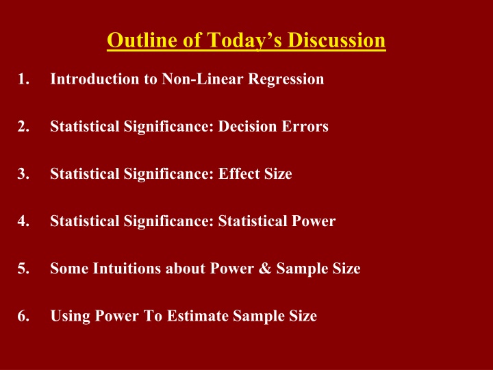
Outline of Todays Discussion 1. Introduction to Non-Linear Regression 2. Statistical Significance: Decision Errors 3. Statistical Significance: Effect Size 4. Statistical Significance: Statistical Power 5. Some Intuitions about Power & Sample Size 6. Using Power To Estimate Sample Size
The Research Cycle Real World Research Representation Abstraction Generalization Methodology *** Data Analysis Research Results Research Conclusions
Part 1 Introduction To Non-linear Regression
Intro to Non-Linear Regression So, far our regression (prediction) has been linear. Graphically, we ve attempted to describe our data with a straight line on a scatter plot. Computationally, we ve used the linear equation: y = mx + b Remember that any mathematical function can be expressed by an equation AND by a picture. Sometimes the relationship between the predictor and the criterion is orderly...BUT NOT LINEAR!
Intro to Non-Linear Regression Polynomial Equations (i.e., many names ) requires estimating one coefficient for each order . In this context, an order is an exponential power. The linear equation is a first order polynomial. Why? y = mx + b The quadratic equation is a second order polynomial. Why? y = ax2 + bx + c Here s a third order polynomial. What would its graph look like? y = ax3 + bx2 + cx + d
Intro to Non-Linear Regression We can compute a correlation coefficient for polynomials or any non-linear equation -just as we did for the simple linear equation. As always, the correlation coefficient (r-statistic) indicates the strength and the direction of the relationship between variables. (The direction is specified by the sign of the highest order coefficient in the polynomial.) As always, the coefficient of determination (r-squared) indicates the proportion of variability in the criterion that is explained by (UGH!) the predictor.
Intro to Non-Linear Regression Higher and higher order polynomials can account for greater and greater proportions of variance (bigger r-squared values). Potential Pop Quiz Question: How does Ockham s razor relate to the use of polynomials in (non-linear) regression analysis?
Intro to Non-Linear Regression Here are a few commonly used non-linear functions (i.e., equations or models ) that differ from the standard polynomial format... y = b * (xm) Power Function: Logarithmic Function: y = m * Ln(x) + b y = b * (em * x) Exponential Function: Slope is controlled by m , intercept is controlled by b . What does the Ln mean? What does e mean? Note: You do NOT need to memorize these formulas!!!
Intro to Non-Linear Regression Great news! We can get the best-fitting non-linear graphs, and the equations, and the r-squared value just by pointing an clicking! Excel to the rescue! Begin by creating a scatter plot in excel, as we ve done before. Select a function, and use the OPTIONS menu to add -display equation on chart -display r-squared value on chart
Part 2 Statistical Significance: Decision Errors
Decision Errors When the right procedure leads to the wrong conclusion Type I Error Reject the null hypothesis when it is true Conclude that a manipulation had an effect when in fact it did not Type II Error Fail to reject the null when it is false Conclude that a manipulation did not have an effect when in fact it did
Decision Errors Setting a strict significance level (e.g., p < .001) Decreases the possibility of committing a Type I error Increases the possibility of committing a Type II error Setting a lenient significance level (e.g., p < .10) Increases the possibility of committing a Type I error Decreases the possibility of committing a Type II error
Part 3 Statistical Significance: Effect Size
Effect Size Potential Pop Quiz Question: If picture c were to be represented on an SPSS output, what would be a plausible sig value? How about an implausible sig value? Explain your answer.
Effect Size There is Trouble in Paradise (Say it with me)
Effect Size 1. One major problem with Null Hypothesis Testing (i.e., inferential statistics) is that the outcome depends on sample size. 2. For example, a particular set of scores might generate a non-significant t-test with n=10. But if the exact same numbers were duplicated (n=20) the t-test suddenly becomes significant . 3. Demo on doubling the sample size
Effect Size 1. Effect Size The magnitude of the influence that the IV has on the DV. 2. Effect size does NOT depend on sample size! ( And there was much rejoicing! )
Effect Size Note: APA recommends reporting an effect size (e.g., Cohen s d, or eta^2) along with the inferential statistic (e.g. t, f, or r stat). This way, we learn whether an effect is reliable (that s what the inferential statistic tells us) and also how large the effect is. (That s what Cohen s d and eta^2 tells us).
Effect Size 1. A statistically significant effect is said to be a reliable effect it would be found repeatedly if the sample size were sufficient. 2. Statistically significant effects are NOT due simply to chance. 3. An effect can be statistically significant, yet puny . 4. There is an important distinction between statistical significance, and practical significance
Effect Size Examples that distinguish effect size and statistical significance . 1. Analogy to a Roulette Wheel An effect can be small, but reliable. 2. Anecdote about the discovery of the planet Neptune - An effect can be small, but reliable. 3. Anecdote about buddy s doctoral thesis, Systematic non-linearities in the production of time intervals . 4. Denison versus Other in S.A.T. scores.
Effect Size Amount that two populations do not overlap The extent to which the experimental procedure had the effect of separating the two groups Calculated by dividing the difference between the two population means by the population standard deviation Effect size conventions Small = .20 Medium = .50 Large = .80
Effect Size Conventions Pairs of population distributions showing a. Small effect size b. Medium effect size c. Large effect size Potential Pop Quiz Question: How would you explain the above graph to a 6th grader?
Effect Size & Meta-Analysis 1. Critical Thinking Question: In your own words, contrast a meta-analysis with a narrative review (from research methods) 2. Critical Thinking Question: In your own words, explain how Cohen s d can be helpful in a meta-analysis.
Effect Size Dividing by the standard deviation standardizes the difference between the means Allows effects to be compared across studies Important tool for meta-analysis Different from statistical significance, which refers to whether an effect is real and not due to chance
Cohens D (Effect Size) Population Mean 1 Population Mean 2 Cohen s D = Population SD It is assumed that Populations 1 and 2 have the same SD.
Small But Reliable Effects Sample: 10,000 verbal SAT test takers whose first name starts with j . Sample Mean = 504 Overall Population Mean = 500 Overall Population SD = 100 Distribution of Means SD2 = Population VAR / n Distribution of Means SD2 = (100^2) / 10,000 = 1 Distribution of Means SD = sqrt(1) = 1 Sample Mean of 504 is 4 z-scores above Population Mean!!!! Reject Ho at the .01 alpha level b/c Z=4 is greater than 2.57, the z-score cut-off at the .01 alpha level, assuming two tails. So, in this case a mean SAT verbal score of 504 is significantly (that is RELIABLY) different from 500 .but does that difference have a practical consequence? NO!!!! Some effects are statistically significant, but are NOT practically significant! Let s compute Cohen s D for this Problem
Small But Reliable Effects Statistical significance is NOT the same thing as effect size. An effect can be puny , yet still statistically significant! Statistical significance is NOT the same thing as practical significance!
Part 4 Statistical Significance: Statistical Power
Statistical Power Probability that a study will produce a statistically significant result if the research hypothesis is true Can be determined from power tables Depends primarily on effect size and sample size More power if Bigger difference between means Smaller population standard deviation More people in the study Also affected by significance level, one- vs. two- tailed tests, and type of hypothesis-testing procedure used
Statistical Power Statistical Power Effect Size Sample Size Cohen s d Noise: Signal: Population Variance Mean Difference
Statistical Power Power = 38% 38% of this distribution (shaded area) falls in the critical region (shaded area) of the comparison distribution. So, we have a 38% chance of rejecting the null and a ( 100 38 = ) 62% chance of NOT rejecting the null. The probability of Type II error is therefore fairly high.
Statistical Power Power = 85% 85% of this distribution (shaded area) falls in the critical region (shaded area) of the comparison distribution. So, we have a 85% chance of rejecting the null and a ( 100 85 = ) 15% chance of NOT rejecting the null. The probability of Type II error is therefore fairly low.
Statistical Power Power = 85% Same story as previous slide but the SD is now half what it was.
Statistical Power Alpha = The probability of a Type I error Beta = The probability of a Type II error (sorry that there are so many Beta s in science!) Power = 1 Beta So, as Beta (probability of Type II error) grows, power decreases. Beta and Power are inversely related.
Statistical Power Remember conceptually Power is the probability that a study will produce a statistically significant result if the research ( alternate ) hypothesis is true! Let s see the preceding slides again and now compute Beta
Statistical Power What does BETA equal here?
Statistical Power What does BETA equal here?
Statistical Power What does BETA equal here?
Statistical Power What does BETA equal here?
Statistical Power What does BETA equal here?
Statistical Power What does BETA equal here?
Statistical Power Two distributions may have little overlap, and the study high power, because a. The two means are very different b. The variance is very small
Increasing Statistical Power Generally acknowledged that a study should have at least 80% power to be worth undertaking Power can be increased by Increasing mean difference Use a more intense experimental procedure Decreasing population SD Use a population with little variation Use standardized measures and conditions of testing Using less stringent significance level Using a one-tailed test instead of two-tailed Using a more sensitive hypothesis-testing procedure
Role of Power in Interpreting the Results of a Study When result is significant If sample size small, effect is probably practically significant as well If sample size large, effect may be too small to be useful When result is insignificant If sample size small, study is inconclusive If sample size large, research hypothesis probably false
Part 5 Some Intuitions About Power & Sample Size
Intuitions About Power & Sample Size An analogy that may help show the relationship among statistical power, and its constituents: Effect Size and Sample Size Let s go fishin


")