Optimal Train Scheduling Research Project Overview
Research project led by Kajal Chokshi and Dr. Grace Guo in the DIMACS REU Summer 2016, funded by NSF and supported by Union Pacific data. Focuses on optimizing train scheduling on single tracks to minimize cost and delay. Utilizes a dataset of 250K records for 6 weeks of single track train schedules to build probability distributions and create empirical distributions using R programming. Visualizes data through various layers and graphs to understand trends and patterns in train behavior on different days and hours of the week.

Download Presentation

Please find below an Image/Link to download the presentation.
The content on the website is provided AS IS for your information and personal use only. It may not be sold, licensed, or shared on other websites without obtaining consent from the author.If you encounter any issues during the download, it is possible that the publisher has removed the file from their server.
You are allowed to download the files provided on this website for personal or commercial use, subject to the condition that they are used lawfully. All files are the property of their respective owners.
The content on the website is provided AS IS for your information and personal use only. It may not be sold, licensed, or shared on other websites without obtaining consent from the author.
E N D
Presentation Transcript
Optimal Train Scheduling Problem Researcher: Kajal Chokshi Mentor: Dr. Grace Guo DIMACS REU Summer 2016 Funded by NSF, Data by Union Pacific
Overview Scheduling trains on single tracks depending on various constraints Various constraints include types of cargo, time of travel, etc. Optimize train schedule in order to minimize cost and delay
Given Information Dataset from a company regarding single track train schedules Approximately 250K records for 6 weeks of data Background information regarding optimization
Dataset Ex. Train Symbol: ACYBAX Train Category: Auto Alpha Origin: Cheyenne Alpha Destination: Barnes Modifier: Extra
Visualize the data using R programming Understand how to build a probability distribution to generate data for simulation Research Goals Optimize train schedule to minimize delay and cost
Methods Visualization through R Programming Analysis of plots and bar graphs Create an Empirical Distribution
Visualization 3 different layers Each layer is a subset of the previous layer Helps understand trends and patterns
Primary Layer Total of 1 graph Purpose: To show train behavior on each day of the week Maximum- Thursday Minimum- Sunday Later end of weekdays tend to have most trains Sunday Monday Tuesday Wednesday Thursday Friday Saturday
Secondary Layer Total of 7 graphs Purpose: To visualize the behavior of trains on an hourly basis Sunday Train does not follow normal distribution, skewed left slightly Most activity between 1 A.M. and 2 A.M. Least activity between 10 A.M. and 11 P.M. followed by 5 A.M. and 6 A.M.
Secondary Layer Graph 2 of 7 Most evenly distributed day Most activity between 9 A.M. and 10 A.M. Least activity between 3 P.M. and 4 P.M. followed by 7 A.M. and 8 A.M. (people coming home and rush hour)
Secondary Layer Graph 3 of 7 Relatively normal distribution Most activity between 1 P.M. and 2 P.M. Least activity between 8 A.M. and 9 A.M. followed by 4 P.M. and 5 P.M. (rush hour and individuals driving home)
Secondary Layer Graph 4 of 7 Wednesday Train follows a closer normal distribution Most activity between 11 A.M. and 12 P.M. Least activity between 6 A.M. and 7 A.M. followed by 3 P.M. and 4 P.M.
Secondary Layer Graph 5 of 7 Relatively normal distribution Most activity between 12 A.M. and 1 A.M. Least activity between 4 A.M. and 5 A.M.
Secondary Layer Graph 6 of 7 Friday Train follows a closer normal distribution Most activity between 11 A.M. and 12 P.M. Least activity between 6 A.M. and 7 A.M.
Secondary Layer Graph 7 of 7 Relatively normal distribution Most activity between 3 A.M. and 4 A.M. Least activity between 5 A.M. and 6 A.M.
Secondary Layer Trends Most activity tends to be in the very early morning or at noon Least activity tends to be during rush hour and the mid afternoon Saturday and Sunday have the most common trends
Tertiary Layer Subset data by Cargo Type Total of 168 graphs
Tertiary Layer Example: Sundays from 1:00 A.M. to 2:00 A.M. Most cargo type: Manifest Least cargo type: Intermodal and Passenger
Tertiary Level Summary Sunday: Monday: Tuesday: Wednesday: Most common cargo type: Local Least common cargo type: Passenger and Special Thursday: Friday: Saturday: Most common cargo type: Manifest Least common cargo type: Intermodal and Passenger Most common cargo type: Manifest Least common cargo type: Passenger Most common cargo type: Manifest and Local Least common cargo type: Passenger and Special Most common cargo type: Manifest Least common cargo type: Passenger, Special, Most common cargo type: Local Least common cargo type: Passenger and Special Most common cargo type: Manifest Least common cargo type: Passenger and Special
Tertiary Level Trends The type of cargo trains to focus on regarding simulating data would be Manifest Local The type of cargo trains to disregard would be Passenger Special
Empirical Distribution Empirical distributions are defined by the data It follows an inverse transformation method Random values are generated during the simulation rather than fitting a theoretical model
Discussion and Conclusion Continuing research using the empirical model Generate data for simulation to no longer require physical data from corporations
Neither a wise man nor a brave man lies down on the tracks of history to wait for the train of the future to run over him. ~Dwight D. Eisenhower Acknowledgements: National Science Foundation DIMACS and Rutgers Dr. Grace Guo
References A. Higgins Optimal Scheduling of Trains On a Single Line Track Ph.D. Thesis, Faculty of Science, Queensland University of Technology (1996) A. Higgins Modelling the Number and Location of Sidings on a Single Line Railway Ph.D. Thesis, Faculty of Science, Queensland University of Technology (1997) Union Pacific Trainline Dataset