Ogata Example: Lag Compensator Design for Type 1 System
Discover how a Lag Compensator design by Ogata helps reduce steady-state error in a Type 1 system, with detailed simulation results and pole analysis. Explore the impact of different damping ratios on system performance and gain calculations for optimal control.

Download Presentation

Please find below an Image/Link to download the presentation.
The content on the website is provided AS IS for your information and personal use only. It may not be sold, licensed, or shared on other websites without obtaining consent from the author. If you encounter any issues during the download, it is possible that the publisher has removed the file from their server.
You are allowed to download the files provided on this website for personal or commercial use, subject to the condition that they are used lawfully. All files are the property of their respective owners.
The content on the website is provided AS IS for your information and personal use only. It may not be sold, licensed, or shared on other websites without obtaining consent from the author.
E N D
Presentation Transcript
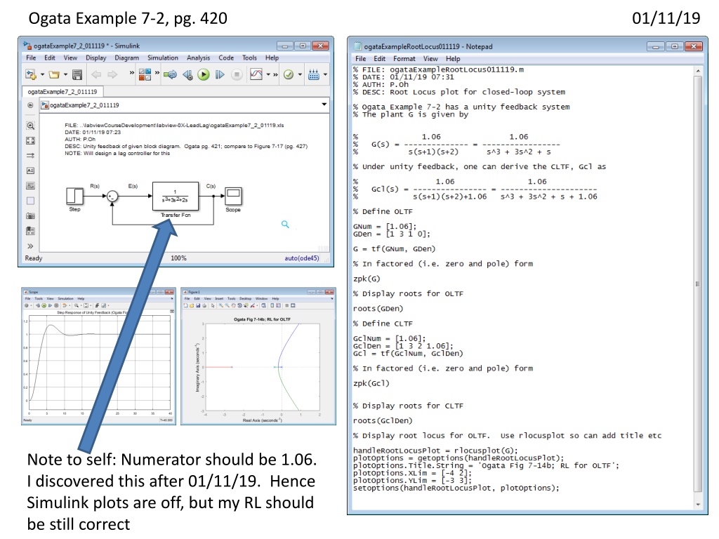
Ogata Example 7-2, pg. 420 01/11/19 Note to self: Numerator should be 1.06. I discovered this after 01/11/19. Hence Simulink plots are off, but my RL should be still correct
01/11/19 Ogata s example is Type 1 system. With unit ramp input, one expects to see steady-state (velocity) error. Output of the Simulink simulation below shows this error is about ??= 0.53 sec 1. This is also 0.53= 1.06 = ??? 1 Unit step: so at 20 sec, output is 20 Output at 20 sec however is 18.08 1 1.92= 0.52 sec 1 Thus error = 20-18.08 = 1.92 or ??=
01/11/19 Using Ogata s Lag Compensator design, the resulting unit ramp input given below Recall that Ogata s design serves to reduce steady-state error 10-times i.e. wants ???= 1.06 0.106 Unit step: so at 20 sec, output is 20 Output at 20 sec however is 20.08 Thus error = 20-20.08 = 0.09 0.1 Close-up of output shows that this was successful
01/11/19 Clicking and dragging on root locus plot shows the pole values for the damping ratio ? = 0.491 that Ogata used. The poles are shown from the plot to be ?1,2= 0.31 ?0.55 like Ogata p. 421
01/11/19 Using the same root locus plot, one can see the poles for different desired pole locations. My understanding is that one can calculate a new gain value in order to have a desired damping ratio e.g. ? = 0.707. I suspect however, that such lag control will cost in poorer steady-state error
01/14/19 From previous slide, we see that for a ? = 0.707, that RL gives us the location of the closed-loop poles. Furthermore, Matlab gives us the gain for that value of poles. Let s calculate the open-loop gain at these poles The OLTF of the compensated system is given by ? + 0.05 ? + 0.005 1.06 ??? ? ? = ?? ?(? + 1)(? + 2) ?(? + 0.05) Where say ? 1.06?? ??? ? ? = Rewrite as ?(? + 0.005)(? + 1)(? + 2) ? = 1 Where just need magnitude at pole locations Recall: 1 + ?? = 0 Hence need ? ?(? + 0.005)(? + 1)(? + 2) (? + 0.05) ( 0.353 + ?0.36)( 0.348 + ?0.36)(0.647 + ?0.36)(1.647 + ?0.36) 0.303 + ?0.36 K = = ?= 0.353+?0.36 ? =(0.504)(0.501)(0.740)(1.685) 0.471 =0.315 0.471= 0.669 1.06=0.669 ? Finally have ??= 1.06= 0.631
01/14/19 1.06=0.669 ? ??= 1.06= 0.631 Left figure: RL from 01/11/19. See from Matlab that Gain of 0.631 same as the ?? calculated above (yellow box)
01/14/19 ( 0.353)2+ 0.362= Recall that ??= 0.353 + ?0.36 = 0.125 + 0.130 0.353 + ?0.36 x = 0.255 = 0.504 ?? 1 ?2 ? =0.353 0.504= 0.700 as expected Hence have ??? 0.353 ?? ?? 1 ?2 ?? ? A formula to recall is: ?0.707 = exp 2.221 ??= exp = exp 3.141 = 0.0432 = 4.3% 0.707 ??? 1 0.5 Note to self: I don t know what ??= 4.3% means physically. Calculations are correct, but the Simulink step response, shows a peak (overshoot) value of 1.175 (suggesting 17.5% overshoot?)
Next time: Understand why Ogata used (?+0.05) (?+0.005) for his lag compensator. I think these values (and/or their ratio) have something to do with reducing steady-state error (by a certain percentage etc).


")