Numerical Study of Submerged Oil Leak Jet

This study focuses on a numerical investigation of a submerged turbulent oil jet, aiming to calculate the oil discharge rate despite the opaque nature of the oil. The research involves experimental test cases, CFD simulations, and analysis of large and small-scale structures in the oil-water interface. The numerical approach utilizes a computational domain, imposed boundary conditions, and a solution technique using OpenFOAM software.

• Numerical Study
• Submerged Oil
• Oil Discharge Rate
• CFD Simulation
• Large-Scale Structures

patr_53 Follow

Uploaded on Nov 14, 2024 | 0 Views

Download Presentation

Please find below an Image/Link to download the presentation.

The content on the website is provided AS IS for your information and personal use only. It may not be sold, licensed, or shared on other websites without obtaining consent from the author. Download presentation by click this link. If you encounter any issues during the download, it is possible that the publisher has removed the file from their server.

Presentation Transcript

1. Driving Innovation Delivering Results Pankaj Saha, Ph.D Numerical Study of Submerged Oil Leak Jet ORISE Research Fellow August 13, 2015 National Energy Technology Laboratory

2. Motivation: An Opaque Jet stream discharging into sea water. Jet is turbulent and oil-water interface shows eddies with different size. How to calculate oil discharge rate? No information inside the Jet core is available due to Opaque Oil. Only option is to use the information of visible large scale features at the outer-edge No reliable correlation available between jet core velocity and outer-edge velocity for multiphase jet. Plan is to pursue lab scale experiment and their CFD simulation to find relationship between outer-edge velocity and jet core velocity. Camera Images of Oil discharge from Macondo wellhead at the bottom of Gulf of Mexico (June 3, 2010). Re=125,000 Deepwater Horizon video clip by Oceaneering National Energy Technology Laboratory 2 International Inc

3. Outline of the Talk Introduction and Motivation Problem Description Numerical Approach Result and Discussion Conclusion National Energy Technology Laboratory 3

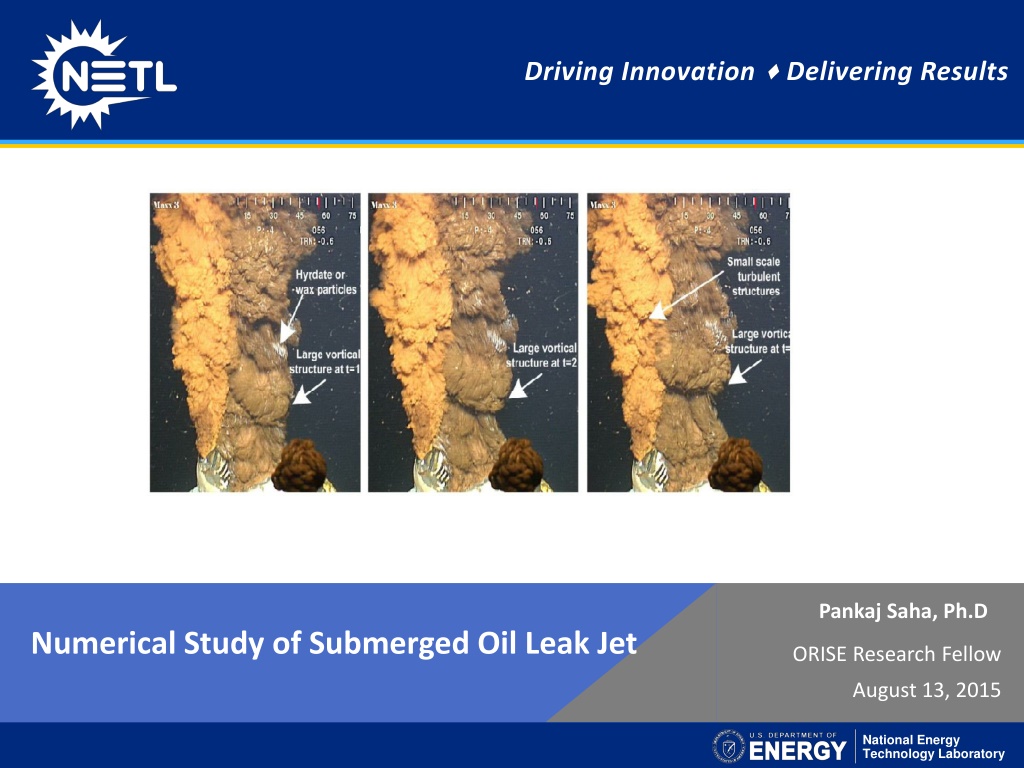
4. Problem Description: Experimental Test Case Experimental Test Case used for CFD Study Video Image of Submerged Turbulent Oil Jet (JP- Fuel) : Experiment done by NETL Group at OHMSETT, Dec , 2014. Oil Jet is Discharged from a long submerged pipe end into Water. Jet Condition at pipe exit is fully turbulent. Flow rate: 270GPM, D=1 , Re=20,000 Properties: 1019kg/m , 1.0x10 m /S = = 3 6 2 w w = = 3 5 2 800kg/m , 4.25x10 m /S oil oil Large Scale spatial Structures Small Scale Turbulence Structures = 0.04N/m Surface Tension: The Images show large and small scale vortices and sharp interfaces National Energy Technology Laboratory 4

5. Numerical Set Up Fully developed turbulent oil jet from exit of circular pipe end discharged into quiescent water . Computational Domain: 25Dx10Dx10D D=Diameter of Jet=1 inch, Re=20,000 Oil-Water properties taken from Experimental flow conditions Imposed Boundary Condition: Jet Inlet: Fully developed realistic turbulent inflow condition All Other Planes: Pressure-Outlet Jet Inlet Schematic of computational domain National Energy Technology Laboratory Energy consumption: DOE EIA, http://www.eia.gov/cfapps/ipdbproject/IEDIndex3.cfm?tid=44&pid=44&aid=2, accessed 12/01/14 GDP: UNDP, http://hdr.undp.org/en/content/gdp-per-capita-2011-ppp, accessed 12/01/14 5

6. Numerical Approach: Solution Technique Numerical package: OpenFOAM, an open source FVM based Unstructured Collocated solver. It has collection of libraries to describe different mathematical terms of the governing fluid flow equations. The libraries are embedded to make a specific Solver Multiphase Incompressible 3D N-S solvers flow solver- interFoam. Single-Fluid Approach- Both the fluids use same set of governing equations. The mixture properties are calculated by volume weighted average based on volume Fraction. Immiscible Oil-Water interface is captured using VOF method. VOF employ High Resolution Interface Capturing convective Scheme (HRIC) to accurately predict the interface. Turbulence is modelled by Large Eddy Simulation (LES) approach LES: One equation eddy model is used. National Energy Technology Laboratory Energy consumption: DOE EIA, http://www.eia.gov/cfapps/ipdbproject/IEDIndex3.cfm?tid=44&pid=44&aid=2, accessed 12/01/14 GDP: UNDP, http://hdr.undp.org/en/content/gdp-per-capita-2011-ppp, accessed 12/01/14 6

7. Numerical Approach: Grid LES needs fine grid to resolve scales upto inertial range. Shear layer and Jet regions need finer grid to resolve fine scales. Hinze relation for dissipation length scale: Re = 3/4 D length scale at inertial sub-range: = /D 60 = /D 27 Re=20000, Grid: 7 M Cells Time Step=10-05 National Energy Technology Laboratory Energy consumption: DOE EIA, http://www.eia.gov/cfapps/ipdbproject/IEDIndex3.cfm?tid=44&pid=44&aid=2, accessed 12/01/14 GDP: UNDP, http://hdr.undp.org/en/content/gdp-per-capita-2011-ppp, accessed 12/01/14 7

8. Turbulent Inlet B.C: Synthetic Turbulence Generator LES needs realistic turbulent inflow at inlet T=0 s Turbulence at Inlet is specified by Synthetic Turbulence Generator. The Technique uses random spot method by using the information of initial velocity profile , stress component and turbulence Intensity. The Technique ensure well spatial and temporal coherence. T=3 s Initial specification of turbulence intensity for inflow generator was calculated using standard pipe flow correlations. Spatial coherent structures Generate spatial coherent Structures The structures does not attenuate over time National Energy Technology Laboratory Energy consumption: DOE EIA, http://www.eia.gov/cfapps/ipdbproject/IEDIndex3.cfm?tid=44&pid=44&aid=2, accessed 12/01/14 GDP: UNDP, http://hdr.undp.org/en/content/gdp-per-capita-2011-ppp, accessed 12/01/14 8

9. Result and Discussion: Stages of Jet Formation Top Fig.: Shows roll up of Shear layer eddies T=0.01 s Bottom Fig.: Shows formation of Jet ligaments, and breaks into smaller size droplets. T=0.04 s Transient development shows Jet leaves the domain in 0.1 Seconds. Flow through Time is ~0.2 Seconds T=0.1 s Iso-Surface of volume Fraction National Energy Technology Laboratory Energy consumption: DOE EIA, http://www.eia.gov/cfapps/ipdbproject/IEDIndex3.cfm?tid=44&pid=44&aid=2, accessed 12/01/14 GDP: UNDP, http://hdr.undp.org/en/content/gdp-per-capita-2011-ppp, accessed 12/01/14 9

10. Result and Discussion: Experimental Validation National Energy Technology Laboratory Energy consumption: DOE EIA, http://www.eia.gov/cfapps/ipdbproject/IEDIndex3.cfm?tid=44&pid=44&aid=2, accessed 12/01/14 GDP: UNDP, http://hdr.undp.org/en/content/gdp-per-capita-2011-ppp, accessed 12/01/14 10

11. Results: Experimental Validation Top: Image of Jet Structures from Exp. Bottom: CFD predicted Jet Structures using iso-surface volume fraction Both the Jet shows similar shapes of small and large scale spatial structures. The Jet expansion angle is also same for both CFD and Experiment(~90 ) Literature provide expansion angle of (10 1) National Energy Technology Laboratory Energy consumption: DOE EIA, http://www.eia.gov/cfapps/ipdbproject/IEDIndex3.cfm?tid=44&pid=44&aid=2, accessed 12/01/14 GDP: UNDP, http://hdr.undp.org/en/content/gdp-per-capita-2011-ppp, accessed 12/01/14 11

12. Results: 3D-Visulization of Jet Instantaneous Jet Structures using iso-surface of volume fraction (0.5) Droplets Formation and striped off from jet Ligament Formation(lobe) National Energy Technology Laboratory Energy consumption: DOE EIA, http://www.eia.gov/cfapps/ipdbproject/IEDIndex3.cfm?tid=44&pid=44&aid=2, accessed 12/01/14 GDP: UNDP, http://hdr.undp.org/en/content/gdp-per-capita-2011-ppp, accessed 12/01/14 12

13. Results: 2D-Visulization at MidPlane through Jet Center Jet Structures using iso-surface of volume fraction at Mid-Plane Shear layer Roll Up and Sheet formation Jet Breaks up into Droplets National Energy Technology Laboratory Energy consumption: DOE EIA, http://www.eia.gov/cfapps/ipdbproject/IEDIndex3.cfm?tid=44&pid=44&aid=2, accessed 12/01/14 GDP: UNDP, http://hdr.undp.org/en/content/gdp-per-capita-2011-ppp, accessed 12/01/14 13

14. Results: Jet Near Field view at MidPlane Contour of volume fraction at Mid-Plane shows Jet Structures VOF Model clearly reproduce sharp interface between Oil and water Sharp Interface with larger wavelength Relatively finer turbulent scale National Energy Technology Laboratory Energy consumption: DOE EIA, http://www.eia.gov/cfapps/ipdbproject/IEDIndex3.cfm?tid=44&pid=44&aid=2, accessed 12/01/14 GDP: UNDP, http://hdr.undp.org/en/content/gdp-per-capita-2011-ppp, accessed 12/01/14 14

15. Results: Jet Near Field view at MidPlane Contour of Velocity and Velocity Vector Finer turbulent scale at the interface Strong inward motion and entrainment of ambient water at interface National Energy Technology Laboratory Energy consumption: DOE EIA, http://www.eia.gov/cfapps/ipdbproject/IEDIndex3.cfm?tid=44&pid=44&aid=2, accessed 12/01/14 GDP: UNDP, http://hdr.undp.org/en/content/gdp-per-capita-2011-ppp, accessed 12/01/14 15

16. Results: Identification of large-Scale turbulent Structures Turbulent Structures are characterize by spatial structures with pure rotation not the shear. Second invariant technique can isolate shear from strain rate tensor, while vorticity cannot. Both the technique identifies large-scale tubular vortical structures at the outer-edge. Downstream no visible structures due to small scale droplets. Unlike Second Invariant, Vorticity technique captures strong shear layer at Jet Inlet, which is not turbulent structures. Large Scale structures posses volume fraction threshold of ~0.4. This volume fraction is used to identify outer edge interface of large scale structures. Convection velocity of these structures is representative of outer-edge velocity. Iso-Surface of Second-invariant Iso-Surface of vorticity National Energy Technology Laboratory Energy consumption: DOE EIA, http://www.eia.gov/cfapps/ipdbproject/IEDIndex3.cfm?tid=44&pid=44&aid=2, accessed 12/01/14 GDP: UNDP, http://hdr.undp.org/en/content/gdp-per-capita-2011-ppp, accessed 12/01/14 16

17. Results: Core Length of primary Jet break Up Contour of Mean Volume Fraction Core Length of Jet primary break up is defined as the axial length where the area of Jet is reduced by 5%. Lc~2D National Energy Technology Laboratory Energy consumption: DOE EIA, http://www.eia.gov/cfapps/ipdbproject/IEDIndex3.cfm?tid=44&pid=44&aid=2, accessed 12/01/14 GDP: UNDP, http://hdr.undp.org/en/content/gdp-per-capita-2011-ppp, accessed 12/01/14 17

18. Results: Turbulence Statistics: Axial Mid Plane Contour of resolved Reynolds Stress Reynolds stresses are dominant in shear layer National Energy Technology Laboratory Energy consumption: DOE EIA, http://www.eia.gov/cfapps/ipdbproject/IEDIndex3.cfm?tid=44&pid=44&aid=2, accessed 12/01/14 GDP: UNDP, http://hdr.undp.org/en/content/gdp-per-capita-2011-ppp, accessed 12/01/14 18

19. Results: Turbulence Statistics: Axial Mid Plane Distribution of Turbulent Kinetic Energy Top: Resolved TKE Bottom: SGS TKE Distribution shows larger turbulent activity in the Shear layer region The turbulence activity are less in the downstream region where droplets are dominant. Suggest fine grid in Shear layer and in initial Jet formation region. Ratio of K_GS/(K_GS+K_SGS)= 85%. Ensures LES is resolving good amount of TKE. And the grid is fine enough. National Energy Technology Laboratory Energy consumption: DOE EIA, http://www.eia.gov/cfapps/ipdbproject/IEDIndex3.cfm?tid=44&pid=44&aid=2, accessed 12/01/14 GDP: UNDP, http://hdr.undp.org/en/content/gdp-per-capita-2011-ppp, accessed 12/01/14 19

20. Results: Turbulence Statistics: Cross-Flow Planes Distribution of Reynolds Stresses at cross- flow planes X=2D Cross-flow Plane Stress are dominated in shear layer. The turbulence is diffusing with the Jet break up and droplet formations X=5D National Energy Technology Laboratory Energy consumption: DOE EIA, http://www.eia.gov/cfapps/ipdbproject/IEDIndex3.cfm?tid=44&pid=44&aid=2, accessed 12/01/14 GDP: UNDP, http://hdr.undp.org/en/content/gdp-per-capita-2011-ppp, accessed 12/01/14 20

21. Results: Turbulence Statistics: Axial Line Plots Velocity fluctuations and turbulent intensity reduces with droplets formation in downstream region. Anisotropy reduces with droplet formation in far field region. Axial Distribution of velocity fluctuations at Jet centerline National Energy Technology Laboratory Energy consumption: DOE EIA, http://www.eia.gov/cfapps/ipdbproject/IEDIndex3.cfm?tid=44&pid=44&aid=2, accessed 12/01/14 GDP: UNDP, http://hdr.undp.org/en/content/gdp-per-capita-2011-ppp, accessed 12/01/14 21

22. Conclusions The Jet expansion angle from CFD agrees with experiment(~90 ) VOF method captures sharp interfaces Large Scale structures are visible in upstream jet region No Visible structures seen in downstream region LES is well resolved Large Scale structures corresponding to volume fraction threshold of ~0.4 , identifies interface of outer edge large scale structures. Core length was found to be twice the diameter of jet. Anisotropy reduces in fully developed jet flow region National Energy Technology Laboratory Energy consumption: DOE EIA, http://www.eia.gov/cfapps/ipdbproject/IEDIndex3.cfm?tid=44&pid=44&aid=2, accessed 12/01/14 GDP: UNDP, http://hdr.undp.org/en/content/gdp-per-capita-2011-ppp, accessed 12/01/14 22

23. Team Members: Frank Shaffer, USDOE National Energy Technology Laboratory Mehrdad Shahnam, USDOE National Energy Technology Laboratory mer Sava , U.C. Berkeley, Department of Mechanical Engineering Dave DeVites, OHMSETT Mar Inc Timothy Steffeck, DOI Bureau of Safety and Environmental Enforcement National Energy Technology Laboratory Energy consumption: DOE EIA, http://www.eia.gov/cfapps/ipdbproject/IEDIndex3.cfm?tid=44&pid=44&aid=2, accessed 12/01/14 GDP: UNDP, http://hdr.undp.org/en/content/gdp-per-capita-2011-ppp, accessed 12/01/14 23

24. Questions? Thanks