Mode Choice and Binary Logit Model Analysis
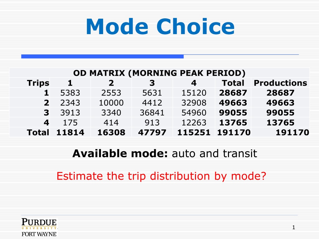


Mode Choice
1
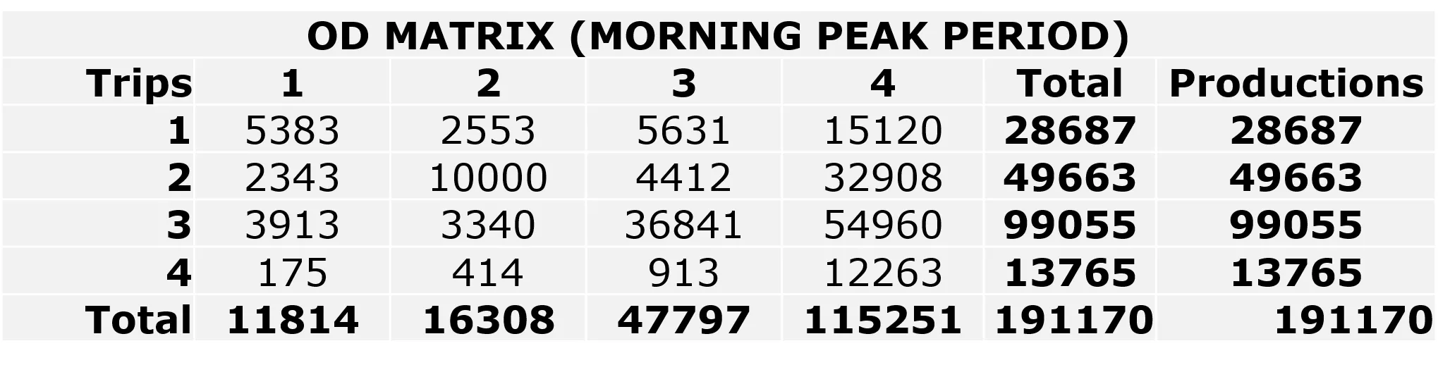
Available mode:
auto and transit
Estimate the trip distribution by mode?

Binary Logit Model
2
U
auto
= 1+0.003*Income/1000-0.04*TravelTime-
0.24*Cost
U
transit
= -3-0.001*Income/1000 -0.04*TravelTime-
0.24*Cost

Example of Binary
Logit Model
3
“In economics,
utility function
is an important
concept that measures preferences over a set
of goods and services.”
Binary Logit Model
4
Probabilities of selecting auto & transit modes:
P
auto ij
= probability of selecting auto mode for trip from TAZ i to TAZ j
U
auto ij
= utility of auto mode for trip from TAZ i to TAZ j: f (auto LOS ij,
auto cost ij, income i…)
P
transit ij
= probability of selecting transit mode for trip from TAZ i to TAZ
j
U
transit ij
= utility of transit mode for trip from TAZ i to TAZ j: f (transit LOS
ij, transit cost ij, income i…)
Travel time and cost
5
Another Example
In-class acitivity
6
Travel characteristics between two zones
U = a
k
– 0.35
t
1
– 0.08
t
2
– 0.005
c
Trip distribution:
total of 12,450 trips going from A
to B
Modal Alternatives
Auto modes
SOV – single occupancy vehicle (drive alone)
HOV – high occupancy vehicle (carpool, vanpool…)
Auto + toll
Transit modes
Bus service (local, express, BRT, intercity)
Rail modes (streetcar, LRT, heavy rail, commuter rail)
Paratransit
Non-motorized modes
Walking, biking…
7
Mode Selection
Attributes
Modal characteristics
LOS, in-vehicle travel times, access time, parking
fee, tolls, transit fare, transfers, convenience,
safety & security, comfort…
Traveler characteristics
Auto availability, HH income, gender, age,
worker/student status, preference…
Area characteristic (build environment)
Density, design, distance to transit,
pedestrian/bike/transit facilities, land use…
8
Another Method
Direct Generation Model
9
Input:
5,000 population, 50 acres
(100 persons/acre)
40% 0 cars/HH
60% 1 car/HH
Source: THE, Garber & Hoel
10
Another method
Trip End Model
Input:
P
TAZ
= 10,000 trips/day
1.80 HHs/auto
15,000 persons/mi
2
In this analysis, the Mode Choice OD Matrix during the Morning Peak Period is examined to estimate trip distributions by mode. A Binary Logit Model is utilized to determine the probabilities of selecting auto and transit modes based on factors such as income, travel time, and cost. Additional information includes examples of how utility functions and probabilities are calculated in the context of transportation planning. Travel characteristics between zones and office & retail space data are also explored.

Download Presentation

Please find below an Image/Link to download the presentation.
The content on the website is provided AS IS for your information and personal use only. It may not be sold, licensed, or shared on other websites without obtaining consent from the author.If you encounter any issues during the download, it is possible that the publisher has removed the file from their server.
You are allowed to download the files provided on this website for personal or commercial use, subject to the condition that they are used lawfully. All files are the property of their respective owners.
The content on the website is provided AS IS for your information and personal use only. It may not be sold, licensed, or shared on other websites without obtaining consent from the author.
E N D
Presentation Transcript
Mode Choice OD MATRIX (MORNING PEAK PERIOD) 2 3 5383 2553 5631 2343 10000 4412 3913 3340 36841 175 414 913 Total 11814 16308 Trips 1 4 Total 28687 49663 99055 13765 Productions 28687 49663 99055 13765 191170 1 2 3 4 15120 32908 54960 12263 115251 191170 47797 Available mode: auto and transit Estimate the trip distribution by mode? 1
Binary Logit Model ???????? ????????+ ??????????? ???????= ??????????= 1 ??????? Uauto = 1+0.003*Income/1000-0.04*TravelTime- 0.24*Cost Utransit = -3-0.001*Income/1000 -0.04*TravelTime- 0.24*Cost 2
Example of Binary Logit Model Passenger Income Travel Time 13 10 10 Cost Mode 1 2 3 - - 40000 60000 80000 $ 3 $ 4 $ 5 Bus Auto Auto In economics,utility function is an important concept that measures preferences over a set of goods and services. 3
Binary Logit Model Probabilities of selecting auto & transit modes: ???????? ????????+ ??????????? ???????= ??????????= 1 ??????? Pauto ij= probability of selecting auto mode for trip from TAZ i to TAZ j Uauto ij = utility of auto mode for trip from TAZ i to TAZ j: f (auto LOS ij, auto cost ij, income i ) Ptransit ij= probability of selecting transit mode for trip from TAZ i to TAZ j Utransit ij = utility of transit mode for trip from TAZ i to TAZ j: f (transit LOS ij, transit cost ij, income i ) 4
Travel time and cost ZONE DATA (CENSUS) Office space (ft^2) 2.00E+06 3.00E+06 1.00E+07 2.50E+07 Retail space (ft^2) 5.00E+06 1.50E+07 1.00E+07 2.00E+07 Zone 1 2 3 4 Households 23,000 35,000 85,000 15,000 Income 30,000 25,000 55,000 85,000 Cars 1.4 1.8 2.5 1.1 Size 2.1 2.2 2.3 1.5 Workers 1.4 1.6 1.5 1.3 ZONE-TO-ZONE TRAVEL TIMES (CAR) 1 2 1 5 13 2 13 5 3 17 25 4 33 15 ZONE-TO-ZONE TRAVEL TIMES (BUS) 1 2 1 13 20 2 20 7 3 35 55 4 45 23 3 17 25 5 14 4 33 15 14 5 3 35 55 10 30 4 45 23 30 5 ZONE-TO-ZONE COSTS (CAR) 1 2 2.75 8.25 8.25 2.75 8.25 13.75 13.75 8.25 ZONE-TO-ZONE TRAVEL COSTS (BUS) 1 2 1 0.75 0.75 2 0.75 0.75 3 0.75 1.25 4 1.25 0.75 3 4 3 4 1 2 3 4 8.25 13.75 2.75 8.25 13.75 8.25 8.25 2.75 0.75 1.25 0.75 0.75 1.25 0.75 0.75 0.75 5
Another Example In-class acitivity Travel characteristics between two zones Variable ak t1 t2 c Auto Transit -0.46 -0.07 20 8 320 30 6 100 U = ak 0.35t1 0.08t2 0.005c Trip distribution: total of 12,450 trips going from A to B 6
Modal Alternatives Auto modes SOV single occupancy vehicle (drive alone) HOV high occupancy vehicle (carpool, vanpool ) Auto + toll Transit modes Bus service (local, express, BRT, intercity) Rail modes (streetcar, LRT, heavy rail, commuter rail) Paratransit Non-motorized modes Walking, biking 7
Mode Selection Attributes Modal characteristics LOS, in-vehicle travel times, access time, parking fee, tolls, transit fare, transfers, convenience, safety & security, comfort Traveler characteristics Auto availability, HH income, gender, age, worker/student status, preference Area characteristic (build environment) Density, design, distance to transit, pedestrian/bike/transit facilities, land use 8
Another Method Direct Generation Model Input: 5,000 population, 50 acres (100 persons/acre) 40% 0 cars/HH 60% 1 car/HH Source: THE, Garber & Hoel 9
Another method Trip End Model Input: PTAZ = 10,000 trips/day 1.80 HHs/auto 15,000 persons/mi2 10